A dual-base station constraint method to improve deformation monitoring precision consistency in strip regions

Abstract

The precision of deformation monitoring with Global Navigation Satellite System (GNSS) relative positioning is significantly influenced by the distance between the monitoring and base stations. In long strip regions, the considerable differences in station spacing lead to inconsistent monitoring precision among multiple stations. This presents a challenge to accurately model and predict the deformation pattern. To tackle this issue, this paper introduces a novel dual-base station constraint method. This method integrates the baseline length constraint between two base stations into the conventional relative positioning model. The formulae of the proposed method are first derived in detail. Then the data collected at eight monitoring stations in two strip regions of 6 km and 8 km over a 28-day period are used to validate the effectiveness of the proposed method. The quantitative analysis of monitoring precision consistency indicators and hypothesis testing on the correlation between monitoring precision and station spacing are conducted. The results show that: (1) median values of the East, North, and Up consistency indicators are reduced from 2.14, 1.41, and 1.83 to 0.91, 0.67, and 0.55 and from 1.85, 1.85, and 2.32 to 0.69, 1.00, and 0.87, respectively, indicating monitoring precision consistency improvement for two case studies; (2) the absolute values of the correlation coefficients between monitoring precision and station spacing decrease from 0.99, 0.94, and 0.98 to 0.09, 0.36, and 0.32. Using the t-test with a significant level of 0.01, it is demonstrated that there is no significant correlation between monitoring precision and station spacing when employing the proposed method.

Introduction

Deformation monitoring is widely needed in various fields, including natural resources (Li et al., 2022), geological disasters (Liu et al., 2022), transportation (Gao et al., 2023), engineering maintenance (Jiang et al., 2022a), and so on. The prevailing deformation monitoring technology is GNSS relative positioning (Wang et al., 2023), which requires at least one base station to achieve mm-level monitoring precision (Han et al., 2018).

With the growing demand for deformation monitoring, Global Navigation Satellite System (GNSS) deformation monitoring has evolved from single monitoring station mode (Zhao et al., 2021) to regional mode with multiple monitoring stations (Huang et al., 2023). In this regional monitoring mode, one major factor affecting monitoring precision is the distance between the base station and the monitoring station (Shi et al., 2017). Based on the spatial distribution of all involved stations, the regional monitoring mode can be further classified into (1) the scenarios with featuring evenly distributed monitoring stations with marginal inter-station spacing differences and (2) the scenarios characterized by unevenly distributed monitoring stations. with significant inter-station spacing difference.

The scenario with evenly distributed monitoring stations is prevalent in most monitoring applications, including landslides, geological hazards, and structural safety (Moschas et al., 2013). In landslide monitoring, the inter-station distance is typically within 5 km (Benoit et al., 2015). Qiu et al. (2018) introduced a novel single-frequency BeiDou Navigation Satellite System (BDS)/Global Positioning System (GPS) monitoring approach, which enhances monitoring precision in landslide-prone areas with a station spacing of approximately 1.0 km. Shi et al. (2019) proposed a GPS relative positioning quality control algorithm. Applying the proposed method to a monitoring station on a tree-surrounded mountain top, mm-level horizontal and cm-level vertical precisions were obtained with 0.7 km inter-station distance. Bai et al. (2019) developed a real-time monitoring and warning cloud platform with mm-level precision, which was successfully deployed in monitoring and issuing warnings for the Heifangtai landslide, where all station spacings were less than 2.0 km. For the same landslide, Wang et al. (2022a) proposed a motion state-constraint base station correction method, resulting in Root Mean Square Errors (RMSEs) of 0.7, 0.9, and 1.5 mm in the East (E), North (N), and Up (U) directions. Carlà et al. (2019) conducted GNSS monitoring on the Super-Sauze landslide in the French Southern Alps, achieving mm-level precision with station spacing less than 1.0 km. In the structure health monitoring applications, the station spacings are typically very close. Jiang et al. (2012) established a GPS monitoring network with station spacing less than 1.0 km, which comprises two base stations and six monitoring stations, achieving mm-level monitoring precision for the Xilongchi reservoir's deformation. Zhang et al. (2019) established a GPS + Galileo (Galileo navigation satellite system) monitoring network on the Forth Road Bridge in Scotland with station spacing from 1.0 km to 1.5 km, achieving the kinematic positioning solution with accuracy at centermeter-decimeter level. Zhang et al. (2020) proposed an improved model with both horizontal and vertical coordinate constraints for the monitoring station. For a 4.4 km baseline, both horizontal and vertical positional precisions were improved from cm to mm level. Vazquez-Ontiveros et al. (2022) accomplished structural health monitoring of the Sanalona Dam using a GNSS monitoring network with station spacing at approximately 2 km, achieving monitoring precision better than 1.0 mm. Xi et al. (2023) constructed a GNSS monitoring network with four monitoring stations approximately separated by 1.3 km, successfully conducting displacement and structural health monitoring of bridges with precision better than 4.0 mm.

The scenarios with non-uniform station distribution often encompass large-scale coverage and long-distance applications. Jiang et al. (2001) scrutinized the impact of tropospheric delay on GPS solution precision, emphasizing the necessity for residual tropospheric error estimation in long-distance monitoring. Bian et al. (2014) undertook extensive monitoring of mining areas using International GNSS (Global Navigation Satellite System) Service (IGS) stations, spaced approximately 35 km apart on average, achieving mm-level monitoring precision. Jiang et al. (2022b) pioneered a BDS automated deformation monitoring system for a long-distance linear water conservancy project, delivering horizontal and vertical monitoring precision of 1.0 and 1.3 mm, respectively. Wang et al. (2022b) proposed a multi-baseline monitoring scheme incorporating prior tropospheric delay constraints to validate its efficacy in enhancing long-distance monitoring performance using GPS/BDS datasets with station spacing of around 20 km. Yuan et al. (2022) found that uneven station distribution affected the precision of positioning results, and the network strength optimization by adding more stations can improve the precision of the weakest points from 3.2 to 2.4 cm. Wang et al. (2024) illustrated that positioning precision of 2 cm horizontally and 3 cm vertically is achievable with station spacing under 30 km in strip GNSS networks.

Another characteristic of long-distance strip applications is the considerable difference in station spacing among multiple monitoring stations, which directly leads to significant disparities in the monitoring precision of these stations. In other words, the consistency among these station’s monitoring precisions is low. Subsequently, this inconsistency issue presents a challenge to accurately model and predict the deformation pattern. Therefore, addressing this issue of monitoring precision inconsistency is imperative in long-distance strip applications.

To address the monitoring precision inconsistency in strip regions, this paper proposes a dual-base station constraint monitoring model, which integrates the baseline length constraint between two base stations into the traditional relative positioning model. The subsequent sections of the paper are structured as follows. The formulae of the proposed method are derived in “Methodology”. “Data description” describes two case studies. “Results and analysis” demonstrates the effectiveness of the proposed method with quantitative analysis of monitoring precision consistency indicators and corresponding hypothesis testing. Finally, “Conclusions” provides concluding remarks.

Methodology

Figure 1 (left) depicts the traditional single-base monitoring network in a strip-shaped region. The base station b₁ is on the western side of the network, and monitoring stations r₁ and r₂ are arranged from west to east. As the base station’s coordinates $\left( {\begin{array}{*{20}c} {X_{{b{}_{1}}} } & {Y_{{b{}_{1}}} } & {Z_{{b{}_{1}}} } \\ \end{array} } \right)^{{\text{T}}}$ are known, we can derive the monitoring station’s coordinate error $\sigma_{r}$ based on the variance–covariance propagation law:

$$ \left( {\begin{array}{*{20}c} {X_{{r_{{}} }} } \\ {Y_{{r_{{}} }} } \\ {Z_{{r_{{}} }} } \\ \end{array} } \right) = \left( {\begin{array}{*{20}c} {X_{{b{}_{1}}} } \\ {Y_{{b{}_{1}}} } \\ {Z_{{b{}_{1}}} } \\ \end{array} } \right) + \left( {\begin{array}{*{20}c} {\Delta X_{{b_{1} ,r}} } \\ {\Delta Y_{{b_{1} ,r}} } \\ {\Delta Z_{{b_{1} ,r}} } \\ \end{array} } \right) \, \Rightarrow \, \left. {\begin{array}{*{20}c} {\sigma_{r}^{2} = \sigma_{{b_{1} }}^{2} + \sigma_{{b_{1} ,r}}^{2} } \\ {\sigma_{{b_{1} }}^{2} = 0} \\ \end{array} } \right\} \, \Rightarrow \, \sigma_{r}^{{}} = \sigma_{{b_{1} ,r}}^{{}} $$

(1)

where $\sigma_{{b_{1} }}$ represents the error of base station coordinates; $\sigma_{{b_{1} ,r}}^{{}} = \alpha^{{}} + \beta^{{}} \times D_{{b_{1} ,r}}^{{}}$ represents the baseline error with $\alpha$ denoting the fixed error, $\beta$ the proportional error, and $D_{{b_{1} ,r}}$ the baseline distance in km.

Fig. 1

Deformation Monitoring Networks: Single-Base vs. Dual-Base Constraint. The left diagram depicts a GNSS monitoring network with single-base station. The right diagram illustrates the deformation monitoring network of the proposed dual-base constraint method. The blue lines represent baselines between base stations and monitoring stations. The red line represents the known baseline between the dual base stations

From Eq. (1), the farther the distance from the base station is, the lower the coordinate precision of the monitoring station will be. For the single-base method shown in Fig. 1 (left), we have $\sigma_{{r_{2} }}^{{}} > \sigma_{{r_{1} }}^{{}}$. This leads to the low consistency issue of the deformation monitoring precision in the strip-shaped regions when using the traditional single-base method.

To tackle the low consistency issue, this study proposes a novel dual-base constraint method. The proposed method involves five steps: (1) construction of the traditional single-base deformation monitoring model; (2) establishment of a dual-base constraint deformation monitoring network; (3) construction of the proposed dual-base constraint monitoring model; (4) repetition of Step (3) to complete the solution for all monitoring stations; and (5) the calculation of the consistency evaluation index and the hypothetical testing on the correlation between the monitoring precision and the inter-station distance.

Step 1: Construction of the traditional single-base monitoring model.

For a short baseline between one base station and one monitoring station, the effects such as ionospheric error, tropospheric delay, and hardware delay can be ignored. The double-differenced observation equation can be obtained as follows:

$$ \left\{ \begin{gathered} \nabla \Delta (P_{i} )_{b,r}^{{S_{{{\text{ref}}}} ,S}} = \nabla \Delta \rho_{b,r}^{{S_{{{\text{ref}}}} ,S}} \hfill \\ \nabla \Delta (L_{i} )_{b,r}^{{S_{{{\text{ref}}}} ,S}} = \nabla \Delta \rho_{b,r}^{{S_{{{\text{ref}}}} ,S}} + \lambda_{i} \nabla \Delta (N_{i} )_{b,r}^{{S_{{{\text{ref}}}} ,S}} \hfill \\ \end{gathered} \right. $$

(2)

where the double-differencing operator is represented by $\nabla \Delta$, the pseudorange observation is denoted by $P$, and the phase observation is denoted by $L$; the subscript i represents the observation frequency, b is the base station, r is the monitoring station; the superscript $S$ denotes the non-reference satellite, while $S_{{{\text{ref}}}}$ represents the reference satellite; $\rho$ signifies the geometric distance between the satellite and the receiver; $\lambda$ represents the wavelength, and $N_{i}$ corresponds to the integer ambiguity.

Linearizing Eq. (2), we can obtain the error equation for the traditional single-base model.

$$ \left\{ {\begin{array}{*{20}c} {\mathop {{\mathbf{V}}_{b,r} }\limits_{2(n - 1) \times 1} = \mathop {{\mathbf{B}}_{b,r} }\limits_{2(n - 1) \times (3 + n - 1)} \times \mathop {{\mathbf{x}}_{b,r} }\limits_{(3 + n - 1) \times 1} - \mathop {{\mathbf{l}}_{b,r} }\limits_{2(n - 1) \times 1} } \\ {{\mathbf{B}}_{b,r} = \left( {\begin{array}{*{20}c} {o_{b,r}^{{S_{{{\text{ref}}}} ,S_{1} }} } & {p_{b,r}^{{S_{{{\text{ref}}}} ,S_{1} }} } & {q_{b,r}^{{S_{{{\text{ref}}}} ,S_{1} }} } & {} & {} & {} \\ \vdots & \vdots & \vdots & {} & {} & {} \\ {o_{b,r}^{{S_{{{\text{ref}}}} ,S_{n - 1} }} } & {p_{b,r}^{{S_{{{\text{ref}}}} ,S_{n - 1} }} } & {q_{b,r}^{{S_{{{\text{ref}}}} ,S_{n - 1} }} } & {} & {} & {} \\ \hline {o_{b,r}^{{S_{{{\text{ref}}}} ,S_{1} }} } & {p_{b,r}^{{S_{{{\text{ref}}}} ,S_{1} }} } & {q_{b,r}^{{S_{{{\text{ref}}}} ,S_{1} }} } & {\lambda_{i} } & {} & {} \\ \vdots & \vdots & \vdots & {} & \ddots & {} \\ {o_{b,r}^{{S_{{{\text{ref}}}} ,S_{n - 1} }} } & {p_{b,r}^{{S_{{{\text{ref}}}} ,S_{n - 1} }} } & {q_{b,r}^{{S_{{{\text{ref}}}} ,S_{n - 1} }} } & {} & {} & {\lambda_{i} } \\ \end{array} } \right),{\mathbf{x}}_{b,r} = \left( {\begin{array}{*{20}c} {{\text{d}}\left( {\Delta X_{b,r} } \right)} \\ {{\text{d}}\left( {\Delta Y_{b,r} } \right)} \\ {{\text{d}}\left( {\Delta Z_{b,r} } \right)} \\ {{\text{d}}[\nabla \Delta (N_{i} )_{b,r}^{{S_{{{\text{ref}}}} ,S_{1} }} ]} \\ \vdots \\ {{\text{d}}[\nabla \Delta (N_{i} )_{b,r}^{{S_{{{\text{ref}}}} ,S_{n - 1} }} ]} \\ \end{array} } \right),{\mathbf{l}}_{b,r} = \left( {\begin{array}{*{20}c} {(P_{i} )_{b,r}^{{S_{{{\text{ref}}}} ,S_{1} }} } \\ \vdots \\ {(P_{i} )_{b,r}^{{S_{{{\text{ref}}}} ,S_{n - 1} }} } \\ \hline {(L_{i} )_{b,r}^{{S_{{{\text{ref}}}} ,S_{1} }} } \\ \vdots \\ {(L_{i} )_{b,r}^{{S_{{{\text{ref}}}} ,S_{n - 1} }} } \\ \end{array} } \right)} \\ \end{array} } \right. $$

(3)

where $S_{1} , \ldots ,S_{n - 1}$ represent $(n - 1)$ non-reference satellites observed; $o_{b,r}^{{S_{{{\text{ref}}}} ,S}} ,p_{b,r}^{{S_{{{\text{ref}}}} ,S}} ,q_{b,r}^{{S_{{{\text{ref}}}} ,S}}$ are the linearization coefficient; ${\text{d}}\left( {{\Delta }X_{b,r} } \right),{\text{d}}\left( {{\Delta }Y_{b,r} } \right),{\text{d}}\left( {{\Delta }Z_{b,r} } \right)$ are the correction terms to the baseline component; $(P_{i} )_{b,r}^{{S_{{{\text{ref}}}} ,S_{1} }}$ and $(L_{i} )_{b,r}^{{S_{{{\text{ref}}}} ,S_{1} }}$ are the misclosure of the linearized pseudorange and phase observation equations, respectively; and ${\mathbf{V}}_{b,r}$ represents the residuals of the pseudorange and phase observations.

With Eqs. (1) and (3), the coordinate precision of the monitoring station for the single-base model can be obtained as:

$$ \left. \begin{gathered} \hat{\sigma }_{0}^{{}} = \sqrt {\frac{{{\mathbf{V}}_{b,r}^{{\text{T}}} {\mathbf{V}}_{b,r} }}{n - 4}} \hfill \\ \sigma_{x\_b,r}^{2} = \hat{\sigma }_{0}^{2} {\mathbf{Q}}_{x\_b,r}^{{}} = \hat{\sigma }_{0}^{2} \left( {{\mathbf{B}}_{b,r}^{{\text{T}}} {\mathbf{B}}_{b,r} } \right)^{ - 1} \hfill \\ \end{gathered} \right\} \Rightarrow \sigma_{{r\_{\text{Single}}}}^{{}} = \sqrt {\frac{{{\mathbf{V}}_{b,r}^{{\text{T}}} {\mathbf{V}}_{b,r} }}{n - 4}{\mathbf{Q}}_{r}^{{}} } $$

(4)

where $\hat{\sigma }_{0}^{{}}$ is the a-posterior unit weight standard deviation; $n - 4$ represents the degrees of freedom; and ${\mathbf{Q}}_{r}^{{}}$ is the cofactor matrix.

Step 2: Establishment of a dual-base constraint monitoring network.

Figure 1 (right) illustrates the deformation monitoring network of the proposed dual-base constraint method. It is an extension of Fig. 1 (left) with the addition of a second base station b₂, positioned to the outsider of the monitoring station r₂. Each monitoring station forms baselines with two base stations, and there is also a known baseline constraint between two base stations.

Step 3: Construction of the proposed dual-base constraint monitoring model.

For the deformation monitoring network consisting of two base stations and one monitoring station, three baselines can be formed: the coordinate difference vector of (b₁, r), (b₂, r) and (b₁, b₂). To facilitate the explanation, it is assumed that all three stations simultaneously observe n satellites. Based on Eq. (3), the error equations of two baselines (b₁, r), (b₂, r) related to the monitoring station r can be obtained as:

$$ \left( {\begin{array}{*{20}c} {{\mathbf{V}}_{{b_{1} ,r}} } \\ \hline {{\mathbf{V}}_{{b_{2} ,r}} } \\ \end{array} } \right)_{{[2(n - 1) + 2(n - 1)] \times 1}} = \left( {\begin{array}{*{20}c} {{\mathbf{B}}_{{b_{1} ,r}} } &\vline & \mathbf{0} \\ \hline \mathbf{0} &\vline & {{\mathbf{B}}_{{b_{2} ,r}} } \\ \end{array} } \right)_{{[2(n - 1) + 2(n - 1)] \times 2\left( {2 + n} \right)}} \times \left( {\begin{array}{*{20}c} {{\mathbf{x}}_{{b_{1} ,r}} } \\ \hline {{\mathbf{x}}_{{b_{2} ,r}} } \\ \end{array} } \right)_{{2\left( {2 + n} \right) \times 1}} - \left( {\begin{array}{*{20}c} {{\mathbf{l}}_{{b_{1} ,r}} } \\ \hline {{\mathbf{l}}_{{b_{2} ,r}} } \\ \end{array} } \right)_{{[2(n - 1) + 2(n - 1)] \times 1}} $$

(5)

Furthermore, a closed loop can be formed among base stations b₁, b₂ and the monitoring station r, such that all three misclosures are equal to zero. This leads to the following three constraint equations:

$$ \left\{ \begin{gathered} 0 = \Delta X_{{b_{1} ,r}} - \Delta X_{{b_{2} ,r}} + \Delta X_{{b_{2} ,b_{1} }} \\ 0 = \Delta Y_{{b_{1} ,r}} - \Delta Y_{{b_{2} ,r}} + \Delta Y_{{b_{2} ,b_{1} }} \\ 0 = \Delta Z_{{b_{1} ,r}} - \Delta Z_{{b_{2} ,r}} + \Delta Z_{{b_{2} ,b_{1} }} \\ \end{gathered} \right. $$

(6)

where $\Delta X_{{b_{1} ,r}} ,\Delta Y_{{b_{1} ,r}} ,\Delta Z_{{b_{1} ,r}}$ and $\Delta X_{{b_{2} ,r}} ,\Delta Y_{{b_{2} ,r}} ,\Delta Z_{{b_{2} ,r}}$ represent the baseline components between b₁, b₂ and r in Eq. (5); $\Delta X_{{b_{2} ,b_{1} }} ,\Delta Y_{{b_{2} ,b_{1} }} ,\Delta Z_{{b_{2} ,b_{1} }}$ represent the baseline components between the two known base stations (b₁, b₂), which can be directly calculated based on their known coordinates $\left( {\begin{array}{*{20}c} {X_{{b_{1} }} } & {Y_{{b_{1} }} } & {Z_{{b_{1} }} } \\ \end{array} } \right)^{{\text{T}}}$ and $\left( {\begin{array}{*{20}c} {X_{{b_{2} }} } & {Y_{{b_{2} }} } & {Z_{{b_{2} }} } \\ \end{array} } \right)^{{\text{T}}}$.

By combining the real observation Eq. (5) and the virtual observation Eq. (6), we can form the proposed dual-base constraint model, namely:

$$ \left( {\begin{array}{*{20}c} {{\mathbf{V}}_{{b_{1} ,r}} } \\ {{\mathbf{V}}_{{b_{2} ,r}} } \\ \hline {{\mathbf{V}}_{r} } \\ \end{array} } \right)_{[2 \times 2(n - 1) + 3] \times 1} = \left( {\begin{array}{*{20}c} {{\mathbf{B}}_{{b_{1} ,r}} } & \mathbf{0} \\ \mathbf{0} & {{\mathbf{B}}_{{b_{2} ,r}} } \\ \hline {{\mathbf{B}}_{r}^{{}} } & { - {\mathbf{B}}_{r}^{{}} } \\ \end{array} } \right)_{{[2 \times 2(n - 1) + 3] \times 2\left( {2 + n} \right)}} \times \left( {\begin{array}{*{20}c} {{\mathbf{x}}_{{b_{1} ,r}} } \\ {{\mathbf{x}}_{{b_{2} ,r}} } \\ \end{array} } \right)_{{2\left( {2 + n} \right) \times 1}} - \left( {\begin{array}{*{20}c} {{\mathbf{l}}_{{b_{1} ,r}} } \\ {{\mathbf{l}}_{{b_{2} ,r}} } \\ \hline {{\mathbf{l}}_{r} } \\ \end{array} } \right)_{[2 \times 2(n - 1) + 3] \times 1} $$

(7)

where ${\mathbf{V}}_{r}$ represents the residual of the virtual observation, ${\mathbf{B}}_{r}$ represents the design matrix of the virtual observation, and ${\mathbf{l}}_{r}$ represents the misclosure of the virtual observation. Their specific expressions are as follows:

$$ \left\{ {\begin{array}{*{20}c} {{\mathbf{B}}_{r} = \left( {\begin{array}{*{20}c} 1 & 0 & 0 & 0 & \cdots & 0 \\ 0 & 1 & 0 & 0 & \cdots & 0 \\ 0 & 0 & 1 & 0 & \cdots & 0 \\ \end{array} } \right)_{3 \times (3 + n - 1)} ,{\mathbf{l}}_{r} = \left( {\begin{array}{*{20}c} {\Delta X_{{b_{1} ,r}}^{0} - \Delta X_{{b_{2} ,r}}^{0} + \Delta X_{{b_{2} ,b_{1} }} } \\ {\Delta Y_{{b_{1} ,r}}^{0} - \Delta Y_{{b_{2} ,r}}^{0} + \Delta Y_{{b_{2} ,b_{1} }} } \\ {\Delta Z_{{b_{1} ,r}}^{0} - \Delta Z_{{b_{2} ,r}}^{0} + \Delta Z_{{b_{2} ,b_{1} }} } \\ \end{array} } \right)_{3 \times 1} } \\ {{\mathbf{x}}_{{b_{j} ,r}} = \left( {\begin{array}{*{20}c} {{\text{d}}\left( {\Delta X_{{b_{j} ,r}} } \right)} & {{\text{d}}\left( {\Delta Y_{{b_{j} ,r}} } \right)} & {{\text{d}}\left( {\Delta Z_{{b_{j} ,r}} } \right)} & {{\text{d}}[\nabla \Delta (N_{i} )_{{b_{j} ,r}}^{{S_{{{\text{ref}}}} ,\;S_{1} }} ]} & \cdots & {{\text{d}}[\nabla \Delta (N_{i} )_{{b_{j} ,r}}^{{S_{{{\text{ref}}}} ,\;S_{n - 1} }} ]} \\ \end{array} } \right)^{{\text{T}}} , \, j{ = 1,2}} \\ \end{array} } \right. $$

(8)

According to the least-squares criterion, the parameters are estimated with Eq. (7) to obtain the baseline vector between (b₁, b₂) and r: $\left( {\begin{array}{*{20}c} {\Delta X_{{b_{1} ,r}} } & {\Delta Y_{{b_{1} ,r}} } & {\Delta Z_{{b_{1} ,r}} } \\ \end{array} } \right)^{{\text{T}}} , \, \left( {\begin{array}{*{20}c} {\Delta X_{{b_{2} ,r}} } & {\Delta Y_{{b_{2} ,r}} } & {\Delta Z_{{b_{2} ,r}} } \\ \end{array} } \right)^{{\text{T}}}$. Substituting the baseline vector into the left side of Eq. (1), we can obtain the coordinates of the monitoring station $(X_{r} ,Y_{r} ,Z_{r} )$:

$$ \left( {\begin{array}{*{20}c} {X_{r} } \\ {Y_{r} } \\ {Z_{r} } \\ \end{array} } \right) = \left( {\begin{array}{*{20}c} {X_{{b_{1} }} } \\ {Y_{{b_{1} }} } \\ {Z_{{b_{1} }} } \\ \end{array} } \right) + \left( {\begin{array}{*{20}c} {\Delta X_{{b_{1} ,r}} } \\ {\Delta Y_{{b_{1} ,r}} } \\ {\Delta Z_{{b_{{_{1} }} ,r}} } \\ \end{array} } \right) \equiv \left( {\begin{array}{*{20}c} {X_{{b_{2} }} } \\ {Y_{{b_{2} }} } \\ {Z_{{b_{2} }} } \\ \end{array} } \right) + \left( {\begin{array}{*{20}c} {\Delta X_{{b_{2} ,r}} } \\ {\Delta Y_{{b_{2} ,r}} } \\ {\Delta Z_{{b_{2} ,r}} } \\ \end{array} } \right) $$

(9)

Since the distance between base stations (b₁, b₂) is known, the equality sign between the middle and the right part of in Eq. (9) indicates that regardless the calculation starts from b₁ or b₂, the obtained coordinates of the monitoring station r are strictly equal.

Combining Eqs. (1) and (7), the precision of the three-dimensional coordinates of the monitoring station r can be obtained as:

$$ \left. \begin{gathered} \hat{\sigma }_{0}^{{}} = \sqrt {\frac{{{\mathbf{V}}_{b,r}^{{\text{T}}} {\mathbf{V}}_{b,r} }}{2n - 5}} \hfill \\ \sigma_{x\_b,r}^{2} = \hat{\sigma }_{0}^{2} {\mathbf{Q}}_{x\_b,r}^{{}} = \hat{\sigma }_{0}^{2} \left( {{\mathbf{B}}_{b,r}^{{\text{T}}} {\mathbf{B}}_{b,r} } \right)^{ - 1} \hfill \\ \end{gathered} \right\} \Rightarrow \, \sigma_{{r\_{\text{Dual}}}}^{{}} = \sqrt {\frac{{{\mathbf{V}}_{b,r}^{\text{T}} {\mathbf{V}}_{b,r} }}{2n - 5}{\mathbf{Q}}_{r}^{{}} } $$

(10)

where $\hat{\sigma }_{0}^{{}}$ represents the a-posterior unit weight standard deviation; $2n - 5$ stands for the degrees of freedom; and ${\mathbf{Q}}_{r}^{{}}$ denotes the cofactor matrix associated with the coordinates of the monitoring station.

Step 4: Repetition of Step 3 to construct the monitoring model for all monitoring stations.

For other monitoring stations $r_{k} \, (k = 2, \ldots ,M)$, repeat Eqs. (7)–(10) to obtain the precision $\sigma_{{r_{k} \_{\text{Dual}}}}^{{}}$ of all monitoring stations.

Step 5: Calculation of the consistency evaluation index and the hypothetical testing on the correlation between the inter-station distance and the monitoring precision.

To assess the consistency in monitoring precision in the strip regions, we designate the monitoring station r₁ closest to the base station b₁ as the reference station (as depicted in Fig. 1). We then calculate the ratio of the precision of each remaining monitoring station to the reference station's precision. This ratio serves as the consistency evaluation index:

$$ R_{{{\text{ratio}}\_r_{i} ,r_{1} }} = \frac{{\sigma _{{r_{i} }} }}{{\sigma _{{r_{1} }} }},{\mkern 1mu} i = 1,2, \ldots ,M $$

(11)

where $\sigma_{{r_{1} }}$ and $\sigma_{{r_{i} }}$ represent the monitoring precisions of r₁ and r_i, respectively. When $R_{{{\text{ratio\_}}r_{i} ,r_{1} }} \approx 1$, it indicates that the precision consistency between r₁ and r_i is high, otherwise, it is low.

In addition to the precision ratio, the monitoring precision consistency in a strip region can also be evaluated by analyzing the correlation between the monitoring precision and the inter-station distance. The Pearson correlation coefficient is used for quantifying the correlation between these two terms by:

$$ p_{{{\text{COR}}}} = \frac{{\sum\limits_{i = 1}^{M} {((D_{{r_{i} }} - \overline{{D_{r} }} )\,(\sigma_{{r_{i} }} - \overline{{\sigma_{r} }} ))} }}{{\sqrt {\sum\limits_{i = 1}^{M} {(D_{{r_{i} }} - \overline{{D_{r} }} )^{2} \,\sum\limits_{I = 1}^{M} {(\sigma_{{r_{i} }} - \overline{{\sigma_{r} }} )^{2} } } } }} $$

(12)

where $p_{{{\text{COR}}}}$ represents the correlation coefficient; $\sigma_{{r_{i} }}$ and $D_{{r_{i} }}$ represent the monitoring precision and inter-station distance, respectively; $\overline{{\sigma_{r} }}$ and $\overline{{D_{r} }}$ represent the average monitoring precision and average inter-station distance of all monitoring stations; M indicates the number of monitoring stations (sample size). A large absolute value of $p_{{{\text{COR}}}}$ indicates a strong correlation between the monitoring precision and the inter-station distance, also suggesting lower monitoring precision consistency in the strip region. Conversely, a small absolute value of $p_{{{\text{COR}}}}$ suggests a weak correlation between precision and inter-station distance, and a high monitoring precision consistency.

To validate the statistical significance of the correlation between the monitoring precision and the inter-station distance, a hypothesis testing is designed as follows.

• (1) Assume the null hypothesis H₀ and the alternative hypothesis H₁.

  $$ H_{0} :p_{{{\text{COR}}}} = 0;\quad H_{1} :p_{{{\text{COR}}}} \ne 0 $$

  (13)

• (2) Construct the test statistic $T_{{{\text{COR}}}}$, which follows a t-distribution with the degrees of freedom $(M - 2)$.

  $$ T_{{{\text{COR}}}} = p_{{{\text{COR}}}} \sqrt {\frac{M - 2}{{1 - p_{{{\text{COR}}}}^{2} }}} t(M - 2) $$

  (14)

• (3) Define a significance level $\alpha_{0}$, and select the critical value $t_{{\alpha_{0} /2}}$ from the statistics table.

  $$ P(|T_{{{\text{COR}}}} |{ > }t_{{\alpha_{0} /2}} ) = \alpha_{0} $$

  (15)

• (4) Compare the calculated statistic and the critical value and make the decision: if $T_{{{\text{COR}}}} > t_{{\alpha_{0} /2}} \,$ or $T_{{{\text{COR}}}} < - t_{{\alpha_{0} /2}}$, then reject H₀ and accept H₁; otherwise, then accept H₀ and reject H₁.

Data description

To evaluate the effectiveness of the proposed method, we employed a 28-day BDS-3 observation dataset for two strip-shaped regions, i.e., day of year (DOY) 149 to 176 in 2023. We calculated deformation monitoring solutions separately using both the traditional single-base method and the innovative dual-base station constraint method proposed herein. Case #1 consisted of three monitoring stations (JC01-JC03) and two base stations (Base1, Base2), while Case #2 comprised five monitoring stations (JC04-JC08) and two base stations (Base1, Base2). As illustrated in Fig. 2, the spatial distribution of all stations conforms to the specific characteristics of the strip-shaped regions.

Fig. 2

Distribution of base and monitoring stations in the strip regions. The left and right diagrams illustrate the respective distributions of GNSS stations for Case #1 and Case #2. In these diagrams, the red pentagons represent base station, while the black dots represent monitoring stations

For the sake of subsequent elaboration, the results and analysis will be demonstrated using the example of a single base station Base1. The solution using Base2 can also reflect the common phenomena. Figure 3 illustrates the monitoring precision for each station in two cases, as well as the inter-station distance to the left base station when using the traditional single-base method. It can be observed that:

• (1) In Case #1, the inter-station distances of JC01 and JC03 are the shortest and longest with 0.8 and 6.7 km, and the corresponding East (E), North (N), and Up (U) monitoring precisions are 1.1, 1.4, and 2.4 mm and 3.1, 2.6, and 5.6 mm, respectively.

• (2) In Case #2, stations JC04 and JC08 have the minimum and maximum inter-station distances of 2.1 and 9.9 km, respectively. The corresponding E, N, and U monitoring precisions are 1.3, 1.5, and 2.1 mm for JC04 and 3.9, 4.1, and 7.9 mm for JC08, respectively.

• (3) Both cases exhibit a noticeable trend of descending monitoring precision with ascending inter-station distance, indicating poor consistency in monitoring precisions.

  Fig. 3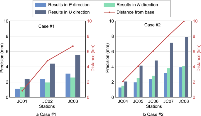

  

  Traditional Single-Base Method: Monitoring Precision and Inter-Station Spacings. The diagram a shows the monitoring precision and inter-station spacings in the E, N, and U directions for Case #1. The diagram b illustrates the monitoring precision and inter-station spacings in the E, N, and U directions for Case #2. In these diagrams, the blue, green, and gray rectangles respectively represent the monitoring precision in the E, N, and U directions, while the red dashed lines indicate inter-station spacings

Results and analysis

As mentioned earlier, the traditional single-base station method exhibits a lack of consistency in monitoring precisions for two strip regions. In the following analysis, we will use these two strip regions as case studies to compare the monitoring precision consistency between the single-base station method and the proposed dual-base station method used. We will elucidate the enhanced effectiveness of our approach in improving the monitoring precision consistency for strip regions.

Case #1

We conducted deformation monitoring of three stations with two approaches: the single-base (Base1) method and the innovative dual-base (Base1 + Base2) constraint method. This enabled us to acquire the deformation time series in the E, N, and U directions. Subsequently, employing a common fitting function, we determined the deformation trend. To evaluate the monitoring precision, we calculated the Root Mean Square (RMS) of the residuals, obtained by subtracting the fitted trend from the original deformation time series.

Taking the farthest monitoring station JC03 from Base1 as an example, Fig. 4 illustrates the solutions obtained using the two methods: the original solution (top row), the fitted trends (middle row), and the fitting residuals (bottom row). It can be observed that:

• (1) Both methods yield the same deformation trend (middle row) in the E, N, and U directions for JC03.

• (2) (2) Deformation series obtained with the conventional single-base method showcases notable fluctuations (top row) in three directions. However, with the implementation of the innovative dual-base constraint method proposed in this study, these fluctuations are marvelously diminished. As a result, the monitoring precision (bottom row) in the E, N, and U direction has been remarkably elevated from 3.1 mm, 2.6 mm, and 5.6 mm to 1.4 mm, 1.5 mm, and 2.6 mm with great improvements by 54.8%, 42.3%, and 53.6%.

  Fig. 4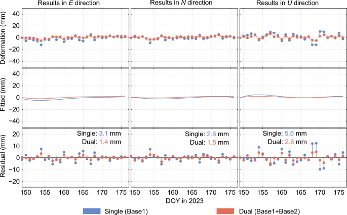

  

  Traditional Single-Base vs. Dual-Base Constraint Solutions for JC03 in Case #1. The blue color indicates the outcomes derived from the single-base method, while the red color represents the outcomes obtained from the proposed dual-base constraint method. The top row displays the original solution, the middle row shows the fitted trends, and the bottom row exhibits the fitting residuals

Monitoring precisions in the E, N, and U directions of all monitoring stations in Case #1 were statistically analyzed using the two methods. The statistical results are presented in Fig. 5. The figure reveals the following insights:

Fig. 5

Case #1: Monitoring precisions in E, N, and U directions—single-base vs. dual-base constraint. The left diagram illustrates the monitoring precision in the E, N, and U directions for each monitoring station when using single-base method in Case #1. The right diagram shows the monitoring precision in the E, N, and U directions for each monitoring station when using the proposed dual-base station constraint method in Case #1. The blue, green, and red rectangles represent the monitoring precision in the E, N, and U directions for JC01, JC02, and JC03, respectively

• (1) With the traditional single-base method, we observe a gradual distance ascent from JC01 to JC03 as they move away from the base station, leading to a gradual descent in monitoring precision. Nevertheless, the dual-base constraint method proposed in this study makes the E, N, and U monitoring precision from JC01 to JC03 remarkable uniformity (right plot), devoid of any apparent correlation with inter-station distance.

• (2) The proposed dual-base constraint method improves monitoring precision in horizontal directions of each monitoring station with a precision better than 2.0 mm and in the vertical direction with a precision better than 4.0 mm. Compared to the results obtained using a single base station (left plot), the proposed dual-base constraint approach enhances the overall monitoring precision in the E, N, and U directions of Case #1.

By taking the E, N, and U monitoring precision of JC01 as the reference, the consistency index for the corresponding direction monitoring precision of all monitoring stations in Case #1 was calculated according to Eq. (11). The results are presented in Table 1 and Fig. 6, which tell the following:

Table 1 Comparison of E, N, and U monitoring precision ratios between the conventional single-base method and the proposed dual-base constraint approach for Case #1 (unitless)

Fig. 6

Monitoring precision ratios comparison: single-base vs. dual-base constraint in case #1. The left diagram illustrates the monitoring precision ratios in the E, N, and U directions for each monitoring station when using single-base method in Case #1. The right diagram shows the monitoring precision ratios in the E, N, and U directions for each monitoring station when using the proposed dual-base station constraint method in Case #1. The blue, green, and red rectangles represent the monitoring precision ratios in the E, N, and U directions for JC01, JC02, and JC03, respectively

• (1) When employing the conventional single-base method, the ratio of monitoring precision gradually increases from JC01 to JC03 in all directions. Notably, JC03 stands out with the largest ratio of 2.79, 1.89, and 2.32 in the E, N, and U directions. However, with the proposed dual-base constraint method, the changes in the ratio of monitoring precision for each direction from JC01 to JC03 become less pronounced and approach to 1.0. Remarkably, the E, N, and U ratio for JC03 decreases significantly to an ideal value of 0.91, 1.09, and 0.85. These findings provide compelling evidence of the efficacy of our approach.

• (2) In contrast to the conventional single-base method, the proposed dual-base constraint method brings the E, N, and U monitoring precision ratios of each station in Case #1 closer to 1.0. This enhancement signifies a notable improvement in the monitoring precision consistency in Case #1.

Case #2

Similarly, we obtained the monitoring results and precisions for five monitoring stations in Case #2. Illustrated in Fig. 7, we specifically showcase the exemplary case of JC08, which stands as the farthest station from Base1. The figure presents the original monitoring results (top row), fitting trend (middle row), and monitoring precision (bottom row) attained with the two distinct monitoring approaches. A similar pattern to the one observed in the previous section emerges for the monitoring station located farthest from the base station (9.9 km), namely:

Fig. 7

Traditional single-base vs. dual-base constraint solutions for JC08 in case #2. The blue color indicates the outcomes derived from the single-base method, while the red color represents the outcomes obtained from the proposed dual-base station constraint method. The top row displays the original solution, the middle row shows the fitted trends, and the bottom row exhibits the fitting residuals

• (1) Two methods reveal an identical deformation trend in the E, N, and U directions for this monitoring station JC08.

• (2) The conventional single-base method yields significant fluctuations in all directions, whereas the proposed dual-base constraint method significantly reduces these fluctuations. As a result, the monitoring precisions in the E, N, and U directions experience an impressive enhancement from 3.9 mm, 4.1 mm, and 7.9 mm to 1.6 mm, 1.8 mm, and 2.5 mm with the improvement by 59.0, 56.1, and 68.4%.

A comprehensive statistical analysis was conducted to assess the monitoring precision in the E, N, and U directions for all stations in Case #2. The results are summarized in Fig. 8. From the figure, Case #2 exhibits similar patterns to Case #1, as follows:

Fig. 8

Case #2: Monitoring precisions in E, N, and U directions—single-base vs. dual-base constraint. The left diagram illustrates the monitoring precision in the E, N, and U directions for each monitoring station when using single-base method in Case #2. The right diagram shows the monitoring precision in the E, N, and U directions for each monitoring station when using the proposed dual-base station constraint method in Case #2. The blue, green, yellow, gray, and red rectangles represent the monitoring precision in the E, N, and U directions for JC04, JC05, JC06, JC07, and JC08, respectively

• (1) With the traditional single-base method, the monitoring precision gradually decreases as the inter-station distance increases from JC04 to JC08. However, the proposed dual-base constraint method does not produce an apparent relationship between the monitoring precision and the inter-station distance from JC04 to JC08.

• (2) By implementing the dual-base constraint method, the monitoring precision remains relatively consistent from JC04 to JC08. In the horizontal directions, all monitoring stations achieve a precision better than 3.0 mm, while the vertical direction precision is better than 4.0 mm. Compared to the solution obtained using the traditional single-base method (left), the proposed dual-base constraint method significantly improves the overall monitoring precision in the E, N, and U directions for Case #2.

In similar to the analysis manner for Case #1 and based on Eq. (11), the consistency indicators for all monitoring stations in Case #2 were calculated with results in Table 2 and Fig. 9. The following findings can be drawn:

Table 2 Comparison of E, N, and U monitoring precision ratios between the traditional single-base method and the proposed dual-base constraint approach for Case #2 (unitless)

Fig. 9

Monitoring Precision Ratios Comparison: Single-Base vs. Dual-Base Constraint in Case #2. The left diagram illustrates the monitoring precision ratios in the E, N, and U directions for each monitoring station when using single-base method in Case #2. The right diagram shows the monitoring precision ratios in the E, N, and U directions for each monitoring station when using the proposed dual-base station constraint method in Case #2. The blue, green, yellow, gray, and red rectangles represent the monitoring precision in the E, N, and U directions for JC04, JC05, JC06, JC07, and JC08, respectively

• (1) With the traditional single-base method, the ratio of monitoring precision gradually increases from JC04 to JC08. JC08 exhibits the largest ratios in all directions, 3.07, 2.66, and 3.82 in E, N, and U, respectively. However, the proposed dual-base constraint method does not change much the precision ratio in each direction from JC04 to JC08, and the ratios are closer to 1.0. In particular, the E, N, and U ratios of JC08 decrease to 0.74, 1.02, and 0.79.

• (2) Compared to the traditional single-base method, the proposed dual-base constraint method also leads to a ratio closer to 1.0 for the monitoring precision in each direction of the stations in Case #2. This indicates an improvement in the monitoring precision consistency in Case #2.

Discussion

To further verify the effectiveness of the proposed method in improving monitoring precision consistency, we will discuss the range and median distributions of consistency indices, as well as the correlation between monitoring precision and inter-station distance in this sub-section.

Range and median of consistency index

The results from Tables 1 and 2 are plotted as boxplots, as shown in Fig. 10. The following patterns can be observed:

Fig. 10

Consistency indices for monitoring precision: single-base method vs. the proposed dual-base constraint method. The left diagram shows the consistency indices of monitoring precision in the E, N, and U directions for Case #1. The right diagram illustrates the consistency indices of monitoring precision in the E, N, and U directions for Case #2. The blue color indicates the outcomes derived from the single-base method, while the red color represents the outcomes obtained from the proposed dual-base constraint method

• (1) In terms of the range, the dual-base constraint method proposed in this study shows smaller ranges compared to the traditional single-base method. Specifically, with the dual-base constraint approach, the longest range of consistency indices is only 0.96 (in Case #2, North), while the range with the single-base method reaches 1.66.

• (2) As for the median values, the medians of consistency indices are closer to 1.0 with the proposed dual-base constraint approach. More specifically, the median value closest to 1.0 among the consistency indices of the single-base method is 1.41 (in Case #1, North). However, with the dual-base constraint approach, the median value for that direction decreases to 1.00.

Considering both the range length and median values, it can be concluded that the proposed dual-base constraint method significantly improves the monitoring precision consistency in a strip region. This ensures that all monitoring stations achieve similar precision without any degradation as the inter-station distance increases.

Correlation analysis between monitoring precision and inter-station distance

By integrating three samples from Fig. 5 and five samples from Fig. 8, we separately computed the correlation coefficient between monitoring precision and inter-station distance using Eq. (12). The results are shown in Table 3 and Fig. 11.

Table 3 Correlation between monitoring precision and inter-station distance for the single-base and the dual-base station constraint approach and their statistics

Fig. 11

Correlation Between Monitoring Precisions and Inter-Station Spacings: Single-Base Method vs. The Proposed Dual-Base Constraint Method. The top row displays the correlation between monitoring precisions and inter-station spacings in the E, N, and U directions when using single-base method. The bottom row shows the correlation between monitoring precisions and inter-station spacings in the E, N, and U directions when using the proposed dual-base station constraint method

In addition, we conducted a hypothesis test to further validate the consistency of our proposed dual-base constraint method using Eqs. (13)–(15). In the hypothesis test, considering a total of eight monitoring stations in the two cases, we determined the t-test statistic: $T_{{{\text{COR}}}} \,t(8 - 2)$. We selected a significant level of 0.01, which corresponds to the two-tailed critical value of 3.707. Numerical results are summarized in Table 3 and illustrated in Fig. 12. It is evident that:

Fig. 12

T-test statistic T_COR of the traditional single-base method and the proposed dual-base station constraint method. The black curve represents the probability density function of the t-distribution with 6 degrees of freedom. The deep red lines represent the critical value for a significance level of 0.01. The two blue regions enclosed by the deep red lines, black curve, and the horizontal axis represent the rejection region of the t-test. The blue and red short lines correspond to the abscissa values, representing the t-test statistics for the single-base method and the proposed dual-base constraint method, respectively

• (1) For the single-base method, the correlation coefficients between E, N, and U monitoring precision and inter-station distance were all above 0.9. Moreover, the absolute values of the t-test statistics for three directions were all larger than 3.707. Both indicate that at the 99% confidence level, we reject the null hypothesis and accept the alternative hypothesis, thereby confirming a strong and highly significant linear correlation between the monitoring precision and the inter-station distance. In other words, the precision consistency is weak.

• (2) As for the proposed dual-base constraint method, the absolute values of the correlation coefficients between monitoring precision and inter-station distance were all less than 0.4. Furthermore, the absolute values (0.221–0.954) of the t-test statistics for the E, N, and U directions were much smaller than the critical value (3.707). From the statistical perspective, we can accept the null hypothesis and reject the alternative hypothesis which means there is no correlation between monitoring precision and inter-station distance.

Indeed, this validates that the dual-base station constraint method proposed in this study enhances the monitoring precision consistency with reducing the correlation between monitoring precision and inter-station distance.

Conclusions

This study proposes a dual-base station constraint method that adds the constraint equations between two base stations to the conventional single-base station model. This proposed method improves the overall monitoring precision of the strip regions, and then enhances the consistency of monitoring precision among all monitoring stations. Furthermore, it essentially eliminates the strong correlation between monitoring precision and inter-station distance. The effectiveness of the proposed method is assessed in two cases with three and five monitoring stations in a period of 28 days in 2023. Some conclusions are derived.

• (1) In Case #1, compared with the traditional single-base method, the proposed method significantly improved the monitoring precision in the E, N, and U directions for the farthest monitoring station from base station by 54.8, 42.3, and 53.6%, respectively. The consistency index in the E, N, and U directions decreased from 2.79, 1.89, and 2.32 to 0.91, 1.09, and 0.85. The proposed method resulted in the consistency indices close to 1.0 for all three monitoring stations.

• (2) In Case #2, the proposed method significantly enhanced the monitoring precision in the E, N, and U directions for the farthest monitoring station compared to the traditional single-base station method. The improvements achieved were remarkable with precision gains of 59.0, 56.1, and 68.4% in the E, N, and U directions, respectively. Moreover, the consistency indices in the E, N, and U directions decreased from 3.07, 2.66, and 3.82 to 0.74, 1.02, and 0.79, indicating a substantial increase in the alignment of monitoring precisions. The proposed method improved the precision consistency of all five monitoring stations, bringing their consistency indices close to 1.0.

• (3) In addition to the improvement of monitoring precision consistency, the proposed method can even eliminate the correlation between monitoring precision and inter-station distance. Compared with the traditional single-base method, the range of the precision consistency indices is shorter, and the median is closer to 1.0. The absolute values of the correlation coefficients between the E, N, and U monitoring precision and the inter-station distance decreased from 0.99, 0.94, and 0.98 to 0.09, 0.36, and 0.32, respectively. This was accompanied by a decrease in the absolute value of the t-statistics for the correlation hypothesis testing, from 14.316, 6.851, and 11.549 (greater than the critical value 3.707) to 0.221, 0.955, and 0.818 (smaller than the critical value 3.707), respectively, implying that no correlation occurred between the monitoring precision and the inter-station distance with the significant level of 0.01.

In summary, the proposed method can enhance precision and improve precision consistency compared to the traditional single-base approach. It effectively eliminates the strong correlation between monitoring precision and inter-station distance. This enhancement facilitates the accurate modeling and prediction of the deformation pattern, thereby enabling more timely warning for monitoring applications in strip regions.

References

Bai, Z., Zhang, Q., Huang, G., Jin, C., & Wang, J. (2019). Real-time BeiDou landslide monitoring technology of “light terminal plus industry cloud.” Acta Geodaetica Et Cartographica Sinica, 48(11), 1424–1429. https://doi.org/10.11947/j.AGCS.2019.20190167
Benoit, L., Briole, P., Martin, O., Thom, C., Malet, J. P., & Ulrich, P. (2015). Monitoring landslide displacements with the Geocube wireless network of low-cost GPS. Engineering Geology, 195, 111–121. https://doi.org/10.1016/j.enggeo.2015.05.020
Bian, H., Zhang, S., Zhang, Q., & Zhang, N. (2014). Monitoring large-area mining subsidence by GNSS based on IGS stations. Transactions of Nonferrous Metals Society of China, 24(2), 514–519. https://doi.org/10.1016/s1003-6326(14)63090-9
Carlà, T., Tofani, V., Lombardi, L., Raspini, F., Bianchini, S., Bertolo, D., & Casagli, N. (2019). Combination of GNSS, satellite InSAR, and GBInSAR remote sensing monitoring to improve the understanding of a large landslide in high alpine environment. Geomorphology, 335, 62–75. https://doi.org/10.1016/j.geomorph.2019.03.014
Gao, R., Liu, Z., Odolinski, R., Zhang, J., Zhang, H., & Zhang, B. (2023). Hong Kong-Zhuhai-Macao Bridge deformation monitoring using PPP-RTK with multipath correction method. GPS Solutions, 27, 195. https://doi.org/10.1007/s10291-023-01491-9
Han, J., Huang, G., Zhang, Q., Tu, R., Du, Y., & Wang, X. (2018). A new azimuth-dependent elevation weight (ADEW) model for real-time deformation monitoring in complex environment by Multi-GNSS. Sensors, 18(8), 2473. https://doi.org/10.3390/s18082473
Huang, G., Du, S., & Wang, D. (2023). GNSS techniques for real-time monitoring of landslides: A review. Satellite Navigation. https://doi.org/10.1186/s43020-023-00095-5
Jiang, W., Chen, Y., Chen, Q., Chen, H., Pan, Y., & Liu, X. (2022a). High precision deformation monitoring with integrated GNSS and ground range observations in harsh environment. Measurement, 204, 112179. https://doi.org/10.1016/j.measurement.2022.112179
Jiang, W., Liang, Y., Yu, Z., Xiao, Y., Chen, Y., & Chen, Q. (2022b). Progress and thoughts on application of satellite positioning technology in deformation monitoring of water conservancy projects. Geomatics and Information Science of Wuhan University, 47(10), 1625–1634. https://doi.org/10.13203/j.whugis20220589
Jiang, W., Liu, H., Liu, W., & He, Y. (2012). CORS development for Xilongchi dam deformation monitoring. Geomatics and Information Science of Wuhan University, 37(8), 949–952.
Jiang, W., Liu, J., & Ye, S. (2001). The systematical error analysis of baseline processing in GPS network. Geomatics and Information Science of Wuhan University, 26(3), 196–199.
Li, X. S., Wang, Y. M., Hu, Y. J., Zhou, C. B., & Zhang, H. (2022). Numerical investigation on stratum and surface deformation in underground phosphorite mining under different mining methods. Frontiers in Earth Science, 10, 14. https://doi.org/10.3389/feart.2022.831856
Liu, K., Geng, J., Wen, Y., Ortega-Culaciati, F., & Comte, D. (2022). Very early post-seismic deformation following the 2015 Mw 8.3 Illapel earthquake, Chile revealed from kinematic GPS. Geophysical Research Letters, 49, e2022GL098526. https://doi.org/10.1029/2022GL098526
Moschas, F., & Stiros, S. (2013). Dynamic multipath in structural bridge monitoring: An experimental approach. GPS Solutions, 18(2), 209–218. https://doi.org/10.1007/s10291-013-0322-z
Qiu, D., Wang, L., Luo, D., Huang, H., Ye, Q., & Zhang, Y. (2018). Landslide monitoring analysis of single-frequency BDS/GPS combined positioning with constraints on deformation characteristics. Survey Review, 51(367), 364–372. https://doi.org/10.1080/00396265.2018.1467-075
Shi, J., Huang, Y., & Ouyang, C. (2019). A GPS relative positioning quality control algorithm considering both code and phase observation errors. Journal of Geodesy, 93(9), 1419–1433. https://doi.org/10.1007/s00190-019-01254-w
Shi, J., Wang, G., Han, X., & Guo, J. (2017). Impacts of satellite orbit and clock on real-time GPS point and relative positioning. Sensors, 17(6), 1363. https://doi.org/10.3390/s17061363
Vazquez-Ontiveros, J. R., Martinez-Felix, C. A., Vazquez-Becerra, G. E., Gaxiola-Camacho, J. R., Melgarejo-Morales, A., & Padilla-Velazco, J. (2022). Monitoring of local deformations and reservoir water level for a gravity type dam based on GPS observations. Advances in Space Research, 69(1), 319–330. https://doi.org/10.1016/j.asr.2021.09.018
Wang, D., Huang, G., Du, Y., Zhang, Q., Bai, Z., & Tian, J. (2023). Stability analysis of reference station and compensation for monitoring stations in GNSS landslide monitoring. Satellite Navigation. https://doi.org/10.1186/s43020-023-00119-0
Wang, D., Huang, G., Du, Y., Bai, Z., Chen, Z., & Li, Y. (2022a). Switching method of GNSS landslide monitoring reference station considering the correction of motion state. Acta Geodaetica Et Cartographica Sinica, 51(10), 2117–2124. https://doi.org/10.11947/j.AGCS.2022.20220295
Wang, H. N., Dai, W. J., & Yu, W. K. (2022b). BDS/GPS multi-baseline relative positioning for deformation monitoring. Remote Sensing, 14(16), 3884. https://doi.org/10.3390/rs14163884
Wang, J., Gao, C., Liu, M., Shang, R., Zhang, R., & Wang, F. (2024). Study on the deployment distance of base station of BDS-3 band CORS system. Engineering of Surveying and Mapping, 33(1), 62–70. https://doi.org/10.19349/j.cnki.issn1006-7949.2024.01.009
Xi, R., Jiang, W., Xuan, W., Xu, D., Yang, J., He, L., & Ma, J. (2023). Performance assessment of structural monitoring of a dedicated high-speed railway bridge using a moving-base RTK-GNSS method. Remote Sensing, 15(12), 3132. https://doi.org/10.3390/rs15123132
Yuan, X., Qing, T., & Zhao, Y. (2022). Analysis of influence of continuous operation reference station selection on GNSS baseline processing accuracy. Engineering of Surveying and Mapping, 31(4), 35–38. https://doi.org/10.19349/j.cnki.issn1006-7949.2022.04.006
Zhang, Q., Ma, C., Meng, X., Xie, Y., Psimoulis, P., Wu, L., Yue, Q., & Dai, X. (2019). Galileo augmenting GPS single-frequency single-epoch precise positioning with baseline constrain for bridge dynamic monitoring. Remote Sensing, 11(4), 438. https://doi.org/10.3390/rs11040438
Zhang, S., Yin, F., Ming, Z., & Li, W. (2020). Real-time kinematic deformation monitoring with prior deformation constraint. Science of Surveying and Mapping, 45(11), 8–12. https://doi.org/10.16251/j.cnki.1009-2307.2020.11.002
Zhao, W. Y., Zhang, M. Z., Ma, J., Han, B., Ye, S. Q., & Huang, Z. (2021). Application of CORS in landslide monitoring. In IOP Conference Series: Earth and Environmental Science (Vol. 861). https://doi.org/10.1088/1755-1315/861/4/042049
Acknowledgements
The authors would like to thank the editor in charge and anonymous reviewers for their valuable comments and suggestions to improve this paper.
Funding
This work has been supported by the National Natural Science Foundation of China (Grant No. 42274050).
Author information
Authors and Affiliations
Contributions
C. Hou processed the experimental data and drafted the manuscript. J. Shi conceptualized and proof-read the manuscript. C. Ouyang revised the manuscript. J. Guo and J. Zou participated in the methodology and result discussion.
Corresponding author
Ethics declarations
Competing interests
The authors declare that they have no known competing financial interests or personal relationships that could have appeared to influence the work reported in this paper.
Additional information
Publisher's Note
Springer Nature remains neutral with regard to jurisdictional claims in published maps and institutional affiliations.
Rights and permissions
Open Access This article is licensed under a Creative Commons Attribution 4.0 International License, which permits use, sharing, adaptation, distribution and reproduction in any medium or format, as long as you give appropriate credit to the original author(s) and the source, provide a link to the Creative Commons licence, and indicate if changes were made. The images or other third party material in this article are included in the article's Creative Commons licence, unless indicated otherwise in a credit line to the material. If material is not included in the article's Creative Commons licence and your intended use is not permitted by statutory regulation or exceeds the permitted use, you will need to obtain permission directly from the copyright holder. To view a copy of this licence, visit http://creativecommons.org/licenses/by/4.0/.
About this article
Cite this article
Hou, C., Shi, J., Ouyang, C. et al. A dual-base station constraint method to improve deformation monitoring precision consistency in strip regions. Satell Navig 5, 26 (2024). https://doi.org/10.1186/s43020-024-00148-3
Received:
Accepted:
Published:
DOI: https://doi.org/10.1186/s43020-024-00148-3