Long-term autonomous time-keeping of navigation constellations based on sparse sampling LSTM algorithm

Abstract

The system time of the four major navigation satellite systems is mainly maintained by multiple high-performance atomic clocks at ground stations. This operational mode relies heavily on the support of ground stations. To enhance the high-precision autonomous timing capability of next-generation navigation satellites, it is necessary to autonomously generate a comprehensive space-based time scale on orbit and make long-term, high-precision predictions for the clock error of this time scale. In order to solve these two problems, this paper proposed a two-level satellite timing system, and used multiple time-keeping node satellites to generate a more stable space-based time scale. Then this paper used the sparse sampling Long Short-Term Memory (LSTM) algorithm to improve the accuracy of clock error long-term prediction on space-based time scale. After simulation, at sampling times of 300 s, 8.64 × 10⁴ s, and 1 × 10⁶ s, the frequency stabilities of the spaceborne timescale reach 1.35 × 10^–15, 3.37 × 10^–16, and 2.81 × 10^–16, respectively. When applying the improved clock error prediction algorithm, the ten-day prediction error is 3.16 × 10^–10 s. Compared with those of the continuous sampling LSTM, Kalman filter, polynomial and quadratic polynomial models, the corresponding prediction accuracies are 1.72, 1.56, 1.83 and 1.36 times greater, respectively.

Introduction

A 1-microsecond time deviation in a navigation satellite can lead to a positioning error of 300 m for users. Therefore, a stable time scale is particularly important for the Global Navigation Satellite System (GNSS) (Tavella, 2008, Tavella & Petit, 2020). Currently, the standard time scale for the four major GNSSs is primarily maintained through multiple high-performance atomic clocks located in timekeeping laboratories. For example, the standard time of the Global Positioning System (GPS) is established and maintained based on atomic clocks from satellites and ground stations, but the weight of satellite clocks is very low. The BeiDou-3 Navigation Satellite System (BDS-3) uses multiple high-performance atomic clocks deployed in ground-based laboratories to generate the standard time scale (Senior & Coleman, 2017). However, this approach relies heavily on ground stations (Zhou et al., 2016), and there is a risk of system service interruption. For example, from July 12th to 17th, 2019, the Galileo navigation satellite system (Galileo) experienced a service interruption of 139 h due to a timing facility failure at the ground control center. The trend for next-generation navigation systems is to use multiple onboard atomic clocks and Inter-Satellite Links (ISLs) to form an in-orbit clock ensemble (Pan et al., 2018; Yang, 2018). Zhou et al. (2023) adopted a scheme to construct a distributed time scale. In this scheme, each satellite uses ISLs to measure clock errors by observing visible satellites in its vicinity. Time synchronization within the constellation is indirectly achieved through time scale algorithm calculations. However, this solution does not truly establish a unified constellation-level timescale. Yang et al. (2023) proposed linking the master clocks carried by each navigation satellite through ISLs to form a large clock group and calculated the constellation-level time scale. However, this solution does not make full use of the backup atomic clocks onboard navigation satellites. We propose a two-level satellite time keeping system and calculate a space-based comprehensive time scale characterized by exceptional stability. In the first-level time keeping system, each navigation satellite carries four atomic clocks to form a small clock ensemble, and the comprehensive time scale for a single satellite is calculated. In the second-level time keeping system, navigation satellites use ISLs to form a large constellation-level clock group, and a space-based comprehensive time scale is calculated. The time scale algorithm can merge multiple atomic clocks into a virtual atomic clock that exhibits better frequency stability (Janis et al., 2021; Wang & Rochat, 2022). Many researchers have proposed different types of time scale algorithms, including the ALGOS algorithm, AT1 algorithm (Manandhar & Meng, 2022; Peng et al., 2019), Kalman filtering algorithm (Greenhall, 2003), Kalman plus Weights (KPW) algorithm (Greenhall, 2001), and wavelet decomposition algorithm (Percival et al., 2012). The KPW time scale algorithm can achieve good real-time performance, and the stability of the output time scale is better. Therefore, we adopt this algorithm to calculate the space-based comprehensive time scale.

During the long-term autonomous operation of a navigation constellation, it is also necessary to maintain time synchronization with the ground time reference. Therefore, accurate forecasting of the clock error of a space-based comprehensive time scale is also important. Common clock error prediction algorithms include linear models, quadratic polynomial prediction algorithms, Kalman prediction algorithms, gray models, and others (Davis et al., 2012). Since space-based atomic clocks are disturbed by factors such as mechanical vibration, electromagnetic radiation, and temperature changes, their clock error prediction models also include nonlinear random terms. Many studies have shown that neural network models have better forecasting effects on nonlinear data (Huang et al., 2021a, 2021b). Among them, the Long Short-Term Memory (LSTM) neural network model exhibits a better forecasting effect on time series data (Greff et al., 2016; Wang et al., 2018). A continuous sampling method was applied to convert the forecast model from a single-variable model into a multivariable forecast model, thereby improving the forecast accuracy of the model. However, since continuous sampling leads to an increase in training samples and cannot best extract the long-term trend items in time series, these methods are less suitable for long-term forecasts of clock errors. Therefore, we use sparse sampling to convert a single-variable model into a multivariable forecast model. This method improves the accuracy of long-term forecasts and reduces the computational complexity.

In this paper, the overall architecture of the autonomous timing scheme for navigation constellations is introduced in Section two. Section three focuses on the simulation and generation of atomic clock data, as well as the principles of time scale algorithms and the improved LSTM algorithm. Section four introduces the experimental simulation and results analysis. Section five presents the conclusions of the article.

Overview of the scheme framework

Currently, research on the time–frequency scheme for the next generation of navigation satellites can be divided into two main directions. Some scholars have proposed starting multiple atomic clocks on a single satellite and forming a small clock group. Although this solution improves the robustness of the single-satellite time scale, it does not study multiple satellites jointly maintain a constellation-level time scale. Other scholars have proposed using ISLs to measure relative clock errors on multiple satellites and generate constellation-level time scale, but they still use the BDS-3 master clock model (only one master clock on a navigation satellite startup); this model does not make full use of all satellite clock resources. Since the next generation of navigation satellites will still be equipped with multiple atomic clocks and laser intersatellite link payloads, we combine the above approaches and propose a two-level space-based time scale generation architecture (a single-satellite clock group and constellation-level clock group). A satellite first generates a more stable single-satellite comprehensive time scale and provides data input for the constellation-level time scale algorithm. Since the model fitting accuracy on single-satellite time scale is higher than that of an atomic clock, so the frequency stability of the final calculated constellation-level time scale is better. This two-level time keeping architecture accounts for both frequency stability and robustness. Figure 1 describes the workflow of the single-satellite time–frequency solution.

Fig. 1

Single-satellite time scale generation architecture

In Fig. 1, the single-satellite clock group is mainly composed of four atomic clocks carried on a timekeeping node satellite. The clock error comparison sequences are input to the time scale algorithm calculation module through the phase comparator, and the single-satellite time scale is calculated as the control reference. The time–frequency control module controls the ultrastable crystal oscillator and outputs physical time–frequency signals (Li, 2019; Wu et al., 2016). Figure 2 describes the constellation-level time scale generation and maintenance architecture.

Fig. 2

Constellation-level time scale generation and maintenance architecture

In Fig. 2, the computing node satellite (a timekeeping node satellite that performs time scale algorithm calculations) obtains the relative clock error between it and each timekeeping node satellite by using ISLs (Yang et al., 2017). Then, the computing node satellite weights and combines multiple single-satellite time scales into a constellation-level comprehensive time scale. By broadcasting the clock error between each satellite and the constellation-level time reference through ISLs, time synchronization of each satellite in the constellation can also be achieved. As time elapses, the relative clock error between the constellation-level time scale and the ground standard time increases, causing the navigation constellation to drift relative to the ground standard clock. The satellite-ground comparison link can be used to regularly measure the satellite-ground clock error data. After modeling and forecasting the satellite-ground clock error, high-precision time synchronization between the satellite and the ground can be achieved.

Methodology

Digital generation of atomic clock data

Modeling and digitally generating atomic clock error data based on their characteristics can provide data input for various time scale algorithms. The clock error model of an atomic frequency standard is as follows (Diez et al., 2006):

$$ x\left( t \right) = x_{0} + y_{0} t + \frac{{Dt^{2} }}{2} + \varepsilon \left( t \right) $$

(1)

where $x_{0}$ is the initial time difference, $y_{0}$ is the initial frequency difference, D is the frequency drift rate, and $\varepsilon \left( t \right)$ is the error term caused by various random noises. Lesson (Leeson, 2016) derived power-law spectral expressions for these noises.

$$ S_{y} \left( f \right) = \sum\limits_{i = - 2}^{i = 2} {\alpha_{i} f^{i} } $$

(2)

where $S_{y} \left( f \right)$ is the spectral density of the atomic clock frequency noise and $\alpha_{i}$ is the intensity coefficient of the five types of noise. The random noise of atomic clocks does not follow a stable normal distribution; therefore, the Allan variance is often used instead of the traditional standard deviation to express the frequency stability of the atomic frequency standard.

$$ \sigma_{y}^{2} (\tau_{m} ) = \frac{1}{2(k - 1)}\sum\limits_{k = 1}^{k - 1} {(\overline{\omega }_{k + 1} - \overline{\omega }_{k} )^{2} } $$

(3)

where $\sigma_{y}^{2} (\tau_{m} )$ represents the Allan variance, $\tau_{m}$ represents the sampling interval, $k$ represents the group sequence number, and $\overline{\omega }_{k}$ is the average value of this group of clock errors. We can use the Allan variance to fit the atomic clock noise coefficient (Zucca et al., 2005). In general, when simulating clock error data, the phase flicker noise can be ignored. In this section, the other four types of noise are simulated, and the final simulated clock error is shown in Formula (4) (Shin et al., 2008):

$$ x(n) = x(n - 1) + (y_{rw} (n) + y_{ff} (n) + y_{wf} (n) + y_{wp} (n))\tau $$

(4)

where $\tau_{{}}$ is the sampling period and $y_{rw}$, $y_{ff}$, $y_{wf}$, and $y_{wp}$ are frequency error terms caused by frequency random walk noise, frequency flicker noise, frequency white noise and phase white noise, respectively.

KPW time scale algorithm

The KPW time scale algorithm first utilizes the Kalman filtering model to forecast the clock error data from multiple atomic clocks. Then, weights are assigned based on the frequency stability of each atomic clock. Finally, multiple atomic clocks are weighted and fused to create a virtual atomic clock (Greenhall, 2001). The Kalman filtering algorithm is a real-time prediction algorithm and can reduce the phase white noise of the system (Davis et al., 2012). Furthermore, atomic clocks with better long-term stability can be assigned larger weights in the time scale algorithm. Therefore, the comprehensive time scale exhibits good long-term and short-term stability, and the KPW time scale algorithm formula is as follows:

$$ x_{e,1} (t) = \sum\limits_{i = 1}^{n} {\omega_{i} (t) \cdot (x_{i,e} (t) - (x_{i,e} (t - \tau ) + \Delta t \cdot \hat{y}_{i,e} (t - \tau ) + 1/2D \cdot (t - \tau )^{2} )} $$

(5)

where $x_{e,1} (t)$ is the clock error of the reference clock relative to the comprehensive time scale, $\tau$ is the sampling period of the clock error data, $x_{i,e}$ is the clock error of each atomic clock relative to the comprehensive time scale, $\hat{y}_{i,e}$ is the forecast of the frequency error of each atomic clock relative to the comprehensive time scale, $D$ represents the frequency drift, and $\omega_{i}$ is the weight allocation array of the clock group (Hutsell, 1996).

LSTM clock error prediction algorithm

The time–frequency characteristics of constellation-level time scale are different from those of current space-based atomic frequency standards. Therefore, its clock error prediction model is also different from traditional clock error prediction models (linear models, quadratic polynomial models, and Kalman filters). Because the LSTM network model can selectively store and forget historical information and maintain long-term memory of past data to better understand trends and patterns in time series data and make more accurate predictions (Xue et al., 2018), we use the LSTM model to perform clock error prediction at the constellation-level time scale. The LSTM algorithm is a special Recurrent Neural Network (RNN) proposed by Hochreiter and recently improved and promoted by Alex Graves (Hochreiter et al., 1997; Greff et al., 2016). Figure 3 shows a schematic diagram of the LSTM algorithm.

Fig. 3

LSTM model framework

As shown in the above architecture diagram, the LSTM algorithm mainly controls four thresholds. $f^{(t)}$ is the forget control unit and is used to select information from the previous round of training to enter the next round of training. $i^{(t)}$ is the input control unit, which determines whether short-term memory information is entered and marked as long-term memory information. $\tilde{c}^{(t)}$ is the selection unit and is used to decide which memories are useful information. $g^{(t)}$ is the output control unit, which is used to determine whether long-term memory can affect short-term memory and control the output of the algorithm (He et al., 2023). LSTM constellation-level time scale clock error prediction involves three main modules: data preprocessing, network model training and forecasting, and data postprocessing. Figure 4 describes the process of LSTM clock error prediction.

Fig. 4

Clock error forecast flow chart

Data preprocessing

• First-order difference: The first-order difference in clock error data can improve the stability of the data, thereby reducing the complexity of the forecasting model and improving the forecasting accuracy (Wang et al., 2016).

• Gross error removal and interpolation: Serious gross errors will affect the accuracy of clock error forecasting. The Median Absolute Deviation (MAD) can indicate gross errors in the data sequence (Huang et al., 2021a, 2021b). After all gross errors are removed, the cubic spline interpolation method can be used to smooth fill in missing values.

• Data splitting: The LSTM algorithm is categorized into single-step prediction and multistep prediction based on the type of input data. The single-step prediction uses multiple historical data points to forecast the next data points, and after obtaining new observation values, the last historical data points are updated before forecasting. The principle of multistep forecasting is to use multiple historical data points to forecast multiple data points. Since new observational clock errors cannot be obtained during the autonomous operation of a constellation, single-step prediction is not suitable for clock error prediction at the constellation-level time scale. Since each forecast value of a multistep forecast will be affected by the previous forecast error, which causes the forecast error to increase rapidly, multistep forecasting is not suitable for long-term forecasts of clock errors at constellation-level time scales. Huang et al., (2021a, 2021b) used the equal interval sampling method to convert a clock error sequence into multiple variables, thereby transforming the clock error multistep forecast model into multiple single-step forecast models and reducing the forecast error. This principle is shown in Fig. 5.

  Fig. 5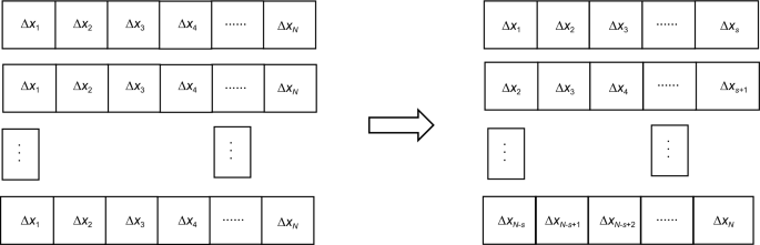

  

  Equally spaced sampling schematic diagram

  The clock error data in each window in Fig. 5 are continuous, so there is a problem of slow divergence of errors in long-term clock error forecasting. We use sparse sampling for data segmentation to improve the ability to remember long-term trend terms during model training, thereby improving the accuracy of long-term clock error forecasts. The clock error data are extracted at every $p$ point to form $N - dp$ windows. This principle is shown in Fig. 6.

  Fig. 6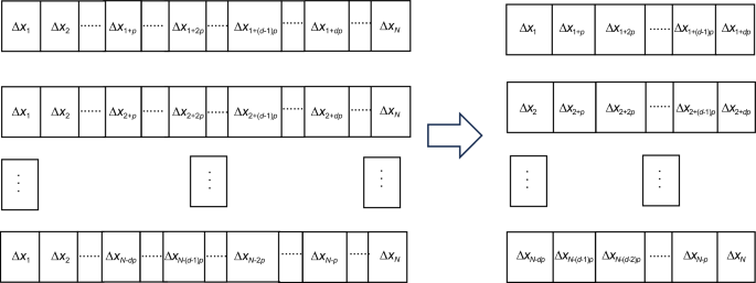

  

  Sparse sampling interval schematic diagram

  As shown in Fig. 6, for the sequence after the first-order difference $\left( {\Delta x_{1} \, \Delta x_{2} \, \cdots \, \Delta x_{N} } \right)$, $p$ is the prediction days, and a matrix of $(N - dp) \times (1 + dp)$ can be generated:

  $$ \left( \begin{gathered} \Delta x_{1} \, \Delta x_{1 + p} \, \Delta x_{1 + 2p} \, \cdots \, \Delta x_{1 + (d - 1)p} \, \Delta x_{1 + dp} \hfill \\ \Delta x_{2} \, \Delta x_{2 + p} \, \Delta x_{2 + 2p} \, \cdots \, \Delta x_{2 + (d - 1)p} \, \Delta x_{2 + dp} \hfill \\ \, \quad\quad\vdots \, \quad\quad\qquad\qquad \ddots \, \quad\quad\quad\quad\vdots \hfill \\ \Delta x_{N - dp} ,\Delta x_{N - (d - 1)p} ,\Delta x_{N - (d - 2)p} ......\Delta x_{N - p} ,\Delta x_{N} \hfill \\ \end{gathered} \right) $$

  (6)

  Parameter d must satisfy Eq. 7:

  $$ d < = \frac{N}{P} - 1 $$

  (7)

  The first d data of each row in the matrix are input to the model as the training sequence, and the optimal d data points are used as training references. After training, the prediction model is obtained. In the prediction stage, the last d data points trained are used as the input set of the prediction stage. The forecast output sequence is $\left( {\Delta x_{{_{1 + (d + 1)p} }} \, \Delta x_{2 + (d + 1)p} \, \Delta x_{3 + (d + 1)p} \, \cdots \, \Delta x_{N + p} } \right)$. The $N - dp$ data outputted by the forecast are obtained from $N - dp$ single-step predictions. Using this method can reduce the accumulation of long-term clock error prediction errors. Compared with continuous sampling, as $p$ increases, the training set also decreases accordingly, thereby reducing the model training time. This article focuses on the selection of the value of $p$. Many simulation experiments were conducted, and it was determined that the best long-term prediction accuracy can be achieved considering the value of $p$.

• Normalize the data: Data normalization can be applied to avoid the impact of different dimensions of each feature quantity and the target value on the prediction performance, accelerate the gradient descent during network training, and increase the convenience of model processing.

Model design and prediction

The LSTM model used in this paper consists of an input layer, a hidden layer, and an output layer. The number of input data points is equal to the number of neurons in the input layer. Each LSTM layer of the hidden layer is connected to a dropout layer, which includes 32 hidden nodes. The dropout layer prevents overfitting during training, and the discard rate is 0.2. Figure 7 illustrates the specific LSTM model structure.

Fig. 7

LSTM model architecture diagram

Table 1 contains the specific parameter settings for the LSTM model.

Table 1 LSTM model parameter list

Data postprocessing

After the LSTM model prediction is complete, the predicted data are denormalized and inversely first-differenced to obtain the predicted clock error sequence. The simulation experiment results and analysis are introduced in detail in the next section.

Simulation and analysis

Clock error data simulation

The specific scenario simulated in this paper is as follows. Each timekeeping node satellite is equipped with 2 passive hydrogen atomic clocks and 2 mercury ion atomic clocks, and there are 6 timekeeping node satellites in the navigation constellation. The hydrogen atomic clock has been applied to the BDS-3 satellite, and its reliability has been verified in advance. Since new satellite-borne atomic clocks, such as mercury ion clocks, have not yet been in orbit for a long time, the stability of the single-satellite times cale was ensured by using hydrogen clocks and high-performance mercury ion clocks to form a small clock group. We downloaded precision clock error data of six BDS-3 hydrogen clocks from the International GNSS Service (IGS) website and obtained frequency stability data of space-based mercury ion clocks tested in orbit (Burt et al., 2021). Then, we used the clock error fitting algorithm introduced earlier to digitally generate 2 sets of clock error data for each hydrogen clock, and based on the stability of the mercury ion clock, we digitally generated 12 sets of clock error data. Since the hydrogen clock and mercury ion clock error data used in our simulation are measured by a satellite-to-ground comparison link, they include errors in the ionosphere and troposphere. Future laser intersatellite links are basically not affected by these errors, so the future clock error measurement noise will be smaller than that in our simulation experiment. Figure 8 shows the stability comparison of each hydrogen clock and the two hydrogen clocks generated by fitting. Figure 9 shows a comparison of the stabilities of the mercury ion clocks and 12 fitted clocks.

Fig. 8

The spectral density was fitted based on the clock error data actually measured by 6 atomic clocks (C26–C30 and C34), and the fitted values were used to simulate the clock error data of 12 hydrogen clocks (H1–H12), the fitting results of six atomic clocks are shown in subfigures a–f respectively

Fig. 9

The clock error data (M1–M12) of 12 mercury ion clocks are simulated based on the fitting values of typical spectral density values of mercury ion clocks

Figures 8 and 9 show that the frequency stability of the simulated atomic clock is very close to that of the actual atomic clock in orbit. Atomic clocks deployed in orbit are affected by periodic noise. Since this periodic noise can be modeled and eliminated through spectral analysis, the clock error simulation in this article does not consider periodic noise.

Constellation-level time scale generation

We set the numbers of 12 hydrogen atomic clocks and 12 mercury ion atomic clocks as H1-H12 and M1-M12, respectively. Two hydrogen clocks and 2 mercury ion clocks on each timekeeping node satellite form a small clock group, and the KPW scale algorithm is employed to calculate the single-satellite time scale (TA1-TA6). Figure 10 shows the frequency stability of each atomic clock and six single-satellite time scales.

Fig. 10

Subfigures a–f show the frequency stability of each atomic clock and single-satellite timescales in the six small clock groups

Figure 10 shows that when the smoothing time is less than 3 × 10⁵ s, all single-satellite timescales are more stable than those of hydrogen atomic clocks or mercury ion clocks. A single satellite clock group consists of two types of atomic clocks, and the number of atomic clocks is small. Therefore, the KPW time scale algorithm cannot effectively suppress frequency flicker noise and frequency random walk noise. Therefore, when the smoothing time is greater than 3 × 10⁵ s, the frequency stabilities of TA2, TA4 and TA6 are between those of the two mercury ion clocks. Each timekeeping node satellite measures the clock error relative to the calculation node satellite through the laser intersatellite link and provides data input for the second-level KPW time scale algorithm. The second-level KPW time scale algorithm outputs the constellation-level time scale TA, and its frequency stability comparison with TA1-TA6 is shown in Fig. 11 and Table 2.

Fig. 11

Constellation-level time scale frequency stability

Table 2 Frequency stability analysis

Figure 11 and Table 2 show that the TA has a better overall advantage than does the single-clock frequency stability or frequency uncertainty. When the averaging interval of the Allan deviation is 300 s, the frequency uncertainty can reach 1.35 × 10^–15, the frequency uncertainty at 1 × 10⁴ s can reach 3.68 × 10^–16, the frequency uncertainty at one day can reach 3.37 × 10^–16, and the frequency uncertainty at 1 × 10⁶ can reach 2.81 × 10^–16. We find that when the smoothing time is 300 s, the frequency uncertainty of the TA is 3.2 times smaller than the average frequency uncertainty of M1-M12 and 15 times smaller than the average frequency uncertainty of H1-H12. When the smoothing time is 1E6, the frequency uncertainty of the TA is 5.1 times smaller than the average frequency uncertainty of M1-M12, and the frequency uncertainty of the TA is 17 times smaller than the average frequency uncertainty of H1-H12. The next section provides a detailed analysis of the simulations of different clock error prediction algorithms.

LSTM-based clock error prediction

First, first-order difference processing is performed on the TA’s original clock error data, and the MAD algorithm is used to determine the gross errors in the data. The gross errors are then smoothed using the cubic spline interpolation algorithm. Figure 12 shows the effect of detecting and processing gross errors.

Fig. 12

Gross error data detection and interpolation, the sampling interval for every epoch is 300 s

In the upper subfigure of Fig. 12, the blue curve represents the first-order difference data of the TA clock error, and the detected gross errors are marked with a red circle. In the lower subfigure of Fig. 12, the green points represent the cubic spline interpolation method-corrected gross error data. Then, the preprocessed first-order difference data are divided, the LSTM network model is trained, and forecasting operation processing is performed. Based on the sparse sampling method introduced in Fig. 6, P = 1,2,…,20, and forecasts are made ten times according to each parameter. Then, the ten forecast errors are averaged, and the forecast error curve is drawn in Fig. 13.

Fig. 13

The average forecast error with different P, the sampling interval is 300 s

Figures 13 and 14 show that when P = 8, the long-term forecast error for more than five days is the smallest. Compared with that of the continuous sampling method with P = 1, the five-day forecast accuracy increases by 75%, and the ten-day forecast accuracy increases by 72%. Let P = 1 and P = 8 be trained and forecasted ten times, respectively; the errors in each forecasting progress are shown in Fig. 15.

Fig. 14

The average forecast error with different P and predicted days

Fig. 15

The forecast error of P = 1 and P = 8, the sampling interval is 300 s

Figure 15 shows that the two values of short-term forecast errors within 6 h are not very different; however, as the forecast time increases, the forecast error at P = 1 diverges faster. However, Fig. 14 also shows that as the P value increases, the forecasting error also tends to increase. Therefore, the reasonable selection of the sampling interval can reduce errors in clock error prediction and model training time. In this paper, P = 8 is selected as the optimal sampling interval by traversing different values. Next, 30 days of historical data are used to predict the clock error of the TA over the next 10 days. Figure 16 and Table 3 show the comparison results for the commonly used Kalman filter forecast algorithm, linear forecast algorithm and Quadratic Polynomial (QP) forecast algorithm.

Fig. 16

The forecast error of different prediction algorithms, the sampling interval is 300 s

Table 3 The statistical result of forecast residual

As shown in Fig. 16 and Table 3, the QP algorithm has the smallest one-day prediction error, which can reach 1.25 × 10^–11 s; the LSTM algorithm has the smallest 5-day prediction error, which can reach 9.30 × 10^–11 s; and the 10-day long-term predicting residual of the LSTM algorithm is also the smallest, which can reach 3.16 × 10^–10 s. In terms of the ten-day forecasting accuracy, the LSTM algorithm is 27% and 36% better than the accuracies of the QP and Kalman algorithms, respectively. Therefore, the LSTM algorithm can be used to make long-term predictions on a constellation-level time scale and improve the level of satellite-ground time synchronization.

Conclusions

To enhance the high-precision autonomous timing capability of next-generation navigation satellites, this paper first proposed a two-level time scale autonomous generation architecture. This architecture not only improves the robustness of the single-satellite time–frequency system but also improves the frequency stability of the space-based time scale. Then we used sparse sampling to transform univariate data into a multivariate LSTM model to improve the accuracy of clock error long-term prediction on space-based time scale. We simulated this solution using 12 hydrogen clocks and 12 mercury ion atomic clocks. When the smoothing times were 300 s, 1 day, and 1E6 s, the corresponding frequency stabilities of the space-based time scale were 1.35 × 10^–15, 3.37 × 10^–16, and 2.81 × 10^–16, respectively. Compared to those of the mercury ion atomic clocks, the frequency stabilities improved by 3.2 times and 15 times when the smoothing time was 300 s and 1 × 10⁶ s, respectively. The 10-day forecast error can reach 3.16 × 10^–10 s. Compared with those of the continuous sampling LSTM, Kalman filter, polynomial and quadratic polynomial models, the corresponding prediction accuracies were 1.72, 1.56, 1.83 and 1.36 times greater, respectively. The research presented in this article has engineering guiding significance for the long-term autonomous timing of future navigation constellations.

The simulation scenario in this article was applied to deploy 6 timekeeping node satellites in a Medium Earth Orbit (MEO) to form a constellation-level clock group. Satellites deployed in the MEO, Geostationary Earth Orbit (GEO) and Inclined GeoSynchronous Orbit (IGSO) have different orbit determination accuracies, relativistic effects and measurement link noise. Therefore, it is necessary to continue to study the impact of deploying timekeeping node satellites in different orbits. Since atomic clocks are easily affected by environmental factors such as mechanical vibration, electromagnetic interference and temperature changes in space, in the future, as the amount of in-orbit data from new atomic clocks increases, we will also conduct research on the impact of these error sources.

References

Burt, E. A., Prestage, J. D., & Tjoelker, R. L. (2021). Demonstration of a trapped-ion atomic clock in space. Nature, 595, 43–47. https://doi.org/10.1038/s41586-021-03571-7
Davis, J., Bhattarai, S., & Ziebart, M. (2012). Development of a Kalman filter based GPS satellite clock time-offset prediction algorithm. 2012 European frequency and time forum (pp. 152–156). https://doi.org/10.1109/EFTF.2012.6502355
Diez, J., D'Angelo, P., & Fernández, A. (2006). Clock errors simulation and characterisation. In Proceedings of the 19th international technical meeting of the satellite division of the institute of navigation (ION GNSS 2006) (pp. 815–821).
Greenhall, C. A. (2001). Kalman plus weights: A time scale algorithm. In Proceedings of the 33th annual precise time and time interval systems and applications meeting (pp. 445–454).
Greenhall, C. A. (2003). Forming stable timescales from the Jones-Tryon Kalman filter. Metrologia, 40(3), S335. https://doi.org/10.1088/0026-1394/40/3/313
Greff, K., Srivastava, R. K., Koutník, J., Steunebrink, B. R., & Schmidhuber, J. (2016). LSTM: A search space odyssey. IEEE Transactions on Neural Networks and Learning Systems, 28(10), 2222–2232. https://doi.org/10.1109/TNNLS.2016.2582924
He, S., Liu, J., Zhu, X., Dai, Z., & Li, D. (2023). Research on modeling and predicting of BDS-3 satellite clock bias using the LSTM neural network model. GPS Solutions, 27(3), 108. https://doi.org/10.1007/s10291-023-01451-3
Hochreiter, S., & Schmidhuber, J. (1997). Long short-term memory. Neural Computation, 9(8), 1735–1780. https://doi.org/10.1162/neco.1997.9.8.1735
Huang, B., Yang, B., Li, M., Guo, Z., Mag, J., & Wang, H. (2021). An improved method for MAD gross error detection of clock error. Geomatics and information science of Wuhan University (accepted for publication). https://doi.org/10.13203/j.whugis20190430
Huang, B., Ji, Z., & Zhai, R. (2021b). Clock bias prediction algorithm for navigation satellites based on a supervised learning long short-term memory neural network. GPS Solutions, 25(2), 80. https://doi.org/10.1007/s10291-021-01115-0
Hutsell, S. T. (1996). Relating the Hadamard variance to MCS Kalman filter clock estimation. In 27th annual precise time and time interval (PTTI) applications and planning meeting (pp. 291–301).
Janis, J. P., Jones, M. R., & Quackenbush, N. F. (2021). Benefits of operating multiple atomic frequency standards for GNSS satellites. GPS Solutions, 25(4), 141. https://doi.org/10.1007/s10291-021-01176-1
Leeson, D. B. (2016). Oscillator phase noise: A 50-year review. IEEE Transactions on Ultrasonics, Ferroelectrics, and Frequency Control. https://doi.org/10.1109/TUFFC.2016.2562663
Li, Y. (2019) Research on High-Precision Time-Frequency Signal Generation and Performance Evaluation. Dissertation, University of Chinese Academy of Sciences
Manandhar, S., & Meng, Y. S. (2022). Study on the effect of using different weighting techniques in a time scale algorithm to generate an ensemble time. In 2022 3rd URSI Atlantic and Asia Pacific Radio Science Meeting (AT-AP-RASC) (pp. 1–4). https://doi.org/10.23919/AT-AP-RASC54737.2022.9814379
Pan, J., Hu, X., Zhou, S., Tang, C., Guo, R., Zhu, L., & Hu, G. (2018). Time synchronization of new-generation BDS satellites using inter-satellite link measurements. Advances in Space Research, 61(1), 145–153. https://doi.org/10.1016/j.asr.2017.10.004
Peng, J. H., Wang, X. L., Fang, J. M., & Wang, Z. P. (2019). Analysis of time scale algorithm in satellite autonomous navigation mode. IOP Conference Series: Earth and Environmental Science, 310(4), 042053. https://doi.org/10.1088/1755-1315/310/4/042053
Percival, D. B., & Senior, K. L. (2012). A wavelet-based multiscale ensemble time-scale algorithm. IEEE Transactions on Ultrasonics, Ferroelectrics and Frequency Control, 59(3), 510–522. https://doi.org/10.1109/TUFFC.2012.2222
Senior, K. L., & Coleman, M. J. (2017). The next generation GPS time. NAVIGATION: Journal of the Institute of Navigation, 64(4), 411–426.
Shin, M. Y., Park, C., & Lee, S. J. (2008). Atomic clock error modeling for GNSS software platform. In 2008 IEEE/ION position, location and navigation symposium (pp. 71–76). https://doi.org/10.1109/PLANS.2008.4570008
Tavella, P. (2008). Statistical and mathematical tools for atomic clocks. Metrologia, 45(6), S183–S192. https://doi.org/10.1088/0026-1394/45/6/S24
Tavella, P., & Petit, G. (2020). Precise time scales and navigation systems: Mutual benefits of timekeeping and positioning. Satellite Navigation, 1, 1–12. https://doi.org/10.1186/s43020-020-00012-0
Wang, Q., & Rochat, P. (2022). ONCLE (One Clock Ensemble) for Galileo’s next-generation robust timing system. Navigation, 69(3), 536. https://doi.org/10.3301/navi.536
Wang, X., Wu, J., Liu, C., Yang, H. Y., Du, Y. L., & Niu, W. S. (2018). Exploring LSTM based recurrent neural network for failure time series prediction. Journal of Beijing University of Aeronautics and Astronautics, 44(4), 772–784.
Wang, Y. P., Lu, Z. P., Zhou, H. T., Wang, N., & Zhai, S. F. (2016). Satellite clock bias prediction based on modified single difference data of clock bias. Journal of Geodesy and Geodynamics, 36(12), 1073–1077.
Wu, Y., Gong, H., Zhu, X., & Ou, G. (2016). A DPLL method applied to clock steering. IEEE Transactions on Instrumentation and Measurement, 65(6), 1331–1342. https://doi.org/10.1109/TIM.2016.2526699
Xue, H., Huynh, D. Q., & Reynolds, M. (2018). SS-LSTM: A hierarchical LSTM model for pedestrian trajectory prediction. In 2018 IEEE winter conference on applications of computer vision (WACV) (pp. 1186–1194). https://doi.org/10.1109/WACV.2018.00135
Yang, D., Yang, J., & Xu, P. (2017). Timeslot scheduling of inter-satellite links based on a system of a narrow beam with time division. GPS Solutions, 21, 999–1011. https://doi.org/10.1007/s10291-016-0587-0
Yang, S., Yi, X., & Dong, R. (2023). A method for autonomous generation of high-precision time scales for navigation constellations. Sensors, 23(3), 1703. https://doi.org/10.3390/s23031703
Yang, Y. (2018). Resilient PNT concept frame. Acta Geodaetica Et Cartographica Sinica, 47(7), 893–898. in Chinese.
Zhou, S., Hu, X., Liu, L., Guo, R., Zhu, L., Chang, Z., & Yu, Y. (2016). Applications of two-way satellite time and frequency transfer in the BeiDou navigation satellite system. Science China Physics, Mechanics & Astronomy, 59, 1–9. https://doi.org/10.1007/s11433-016-0185-6
Zhou, W., Gao, W., Pan, J., Hu, X., Zhou, S., Shao, R., & Yuan, Y. (2023). Analysis of preliminary results from distributed autonomous timekeeping on Beidou-3 satellites. GPS Solutions, 27(2), 80.
Zucca, C., & Tavella, P. (2005). The clock model and its relationship with the Allan and related variances. IEEE Transactions on Ultrasonics Ferroelectrics & Frequency Control, 52(2), 289–296. https://doi.org/10.1109/TUFFC.2005.1406554
Acknowledgements
Thanks Dr. Liu Jiulong of Sun Yat-sen University for his support and guidance on experimental simulation.
Funding
This research was funded by the National Natural Science Foundation of China Youth Project (Grant No. 12104485). Additionally, it has received funding support from the basic research project of Microsatellite Innovation Institute, Chinese Academy of Sciences with grant number JCZX2022B-03.
Author information
Authors and Affiliations
Contributions
SY, WG and RD proposed the experimental plan of the paper, SY and XY wrote the paper content, YW modified the English description of the article and optimized the image quality, QR provided theoretical guidance for the time scale algorithm, TS provided clock error data and made preprocessing suggestions for the data. JZ provided optimization suggestions for the structure of this article.
Corresponding author
Ethics declarations
Competing interests
The authors declare that they have no competing interests.
Additional information
Publisher's note
Springer Nature remains neutral with regard to jurisdictional claims in published maps and institutional affiliations.
Rights and permissions
Open Access This article is licensed under a Creative Commons Attribution 4.0 International License, which permits use, sharing, adaptation, distribution and reproduction in any medium or format, as long as you give appropriate credit to the original author(s) and the source, provide a link to the Creative Commons licence, and indicate if changes were made. The images or other third party material in this article are included in the article's Creative Commons licence, unless indicated otherwise in a credit line to the material. If material is not included in the article's Creative Commons licence and your intended use is not permitted by statutory regulation or exceeds the permitted use, you will need to obtain permission directly from the copyright holder. To view a copy of this licence, visit http://creativecommons.org/licenses/by/4.0/.
About this article
Cite this article
Yang, S., Yi, X., Dong, R. et al. Long-term autonomous time-keeping of navigation constellations based on sparse sampling LSTM algorithm. Satell Navig 5, 15 (2024). https://doi.org/10.1186/s43020-024-00137-6
Received:
Accepted:
Published:
DOI: https://doi.org/10.1186/s43020-024-00137-6