Machine learning based GNSS signal classification and weighting scheme design in the built environment: a comparative experiment

Abstract

None-Line-of-Sight (NLOS) signals denote Global Navigation Satellite System (GNSS) signals received indirectly from satellites and could result in unacceptable positioning errors. To meet the high mission-critical transportation and logistics demand, NLOS signals received in the built environment should be detected, corrected, and excluded. This paper proposes a cost-effective NLOS impact mitigation approach using only GNSS receivers. By exploiting more signal Quality Indicators (QIs), such as the standard deviation of pseudorange, Carrier-to-Noise Ratio (C/N₀), elevation and azimuth angle, this paper compares machine-learning-based classification algorithms to detect and exclude NLOS signals in the pre-processing step. The probability of the presence of NLOS is predicted using regression algorithms. With a pre-defined threshold, the signals can be classified as Line-of-Sight (LOS) or NLOS. The probability of the occurrence of NLOS is also used for signal subset selection and specification of a novel weighting scheme. The novel weighting scheme consists of both C/N₀ and elevation angle and NLOS probability. Experimental results show that the best LOS/NLOS classification algorithm is the random forest. The best QI set for NLOS classification is the first three QIs mentioned above and the difference of azimuth angle. The classification accuracy obtained from this proposed algorithm can reach 93.430%, with 2.810% false positives. The proposed signal classifier and weighting scheme improved the positioning accuracy by 69.000% and 40.700% in the horizontal direction, 79.361% and 75.322% in the vertical direction, and 75.963% and 67.824% in the 3D direction.

Introduction

Demand for mission-critical transportation and logistics services is increasing rapidly, particularly in urban areas. These services, by definition, require high-performance levels from systems that provide Positioning, Navigation, and Timing (PNT). Taking the example of services needed to support autonomous vehicles, the Society of Automotive Engineers (SAE) specifies the six levels of automation in Fig. 1 (SAE International, 2018). These levels range from 0 (full manual driving) to 5 (fully autonomous driving). At present, self-driving vehicles are transitioning from Level 3 to Level 4. Level 3 vehicles can detect the road environment and then make decisions by themselves, such as cruising at a fixed velocity on a highway. For example, Audi A8L equipped with the Traffic Jam Pilot (TJP) technology was unveiled in 2019 and certified in Germany as Level 3 (Saber et al., 2021). However, drivers must be prepared to take over vehicle control when accidents occur or the autonomous driving system fails.

Fig. 1

Society of automotive engineers levels of vehicle autonomy (source: National Highway Traffic Safety Administration)

Compared to Level 3, Level 4 vehicles can control themselves when the aforementioned emergencies occur. Thus, Levels 3 and 4 are also known as the fail-safe and fail-operational levels, respectively. Example Level 4 vehicles currently being tested are Alphabet's Waymo, Baidu's Apollo, Magna's MAX4, and NAVYA. To achieve a high degree of positioning accuracy (decametric or better) with high availability, multi-sensor integration, including the Global Navigation Satellite System (GNSS), is commonly implemented.

GNSS comprises four global, two regional, and several augmentation systems. Starting with GPS many years ago, the development and operation of the additional systems resulted in receiving many more GNSS signals simultaneously (Li et al., 2020). For example, Fig. 2 shows that a U-blox receiver can receive more than 20 signals from the various systems at Imperial College London. Even with GPS and GLONASS, more than ten signals can be received and used for PNT. However, using all multi-constellation signals for positioning and navigation, particularly in built-up areas, increases the computational burden and the possibility of significant and unacceptable measurement errors. Such measurements should be detected and, where possible, excluded. Hence, the main tasks are to detect and exclude faulty signals, enabling the use of the best signals subset. Failure Detection and Exclusion (FDE) should ideally be designed to be used across the entire signal processing chain, including pre-processing and the positioning, navigation, and timing functions. This paper uses machine learning algorithms together with GNSS measurement Quality Indicators (QIs) for FDE in the pre-processing function.

Fig. 2

(Source: U-blox U-center 2)

GNSS signal reception in imperial college, London

From the generation of the data message, upload to GNSS satellites to transmission, reception of GNSS signals, and processing them in receivers, these signals are contaminated by error sources listed in Table 1 (Hofmann-Wellenhof, Lichtenegger & Wasle, 2007; Kaplan & Hegarty, 2005). Among these error sources, multipath occurs when the direct signal and its reflection are received together. Especially from a geometric perspective in the built environment, if the signal paths are shaded, the signals are reflected by static and dynamic objects and received by the receiver, resulting in large measurement errors. The signals that can be received directly are referred to as Line-of-Sight (LOS). Instead, we collectively denote reflected and multipath signals None-Line-of-Sight (NLOS).

Table 1 Main GNSS error sources

As the multipath error in the L1 pseudorange and carrier phase can reach 450 m, and a quarter of the wavelength, which is approximately 5 cm, respectively (European Space Agency, 2013), LOS signals have relatively small pseudorange errors (metre level) compared to NLOS signals. Thus, the QI relative to pseudorange error characteristics can be used to detect NLOS signals.

Like the PNT requirements for autonomous driving, the multipath error also depends greatly on the surrounding physical environment influencing traffic scenarios. In an open area, almost all GNSS signals can be received directly from satellites. However, there is a wide variety of complex environmentally influenced traffic scenarios such as in the urban canyon, semi-urban, suburb, viaducts, boulevards, and tunnels (Wang, Groves & Ziebart, 2015). In the urban canyon, GNSS signals can be blocked or reflected by high-rise buildings, trees, and other static or dynamic obstacles. These obstacles could result in severe multipath errors, resulting in unacceptable position errors, which cannot be mitigated through differential techniques (MacGougan et al., 2002; Ward, 1997). NLOS pseudorange measurement errors can also be large (Hsu et al., 2017). Therefore, the NLOS signals are regarded as faulty signals in this paper. The multipath impact can be mitigated by detecting and excluding the NLOS signals or reducing the weight of these signals.

Several methods have been proposed to mitigate the effect of NLOS signals, including improved antenna and receiver design, use of weighting models or statistical approaches, signal processing, consistency checking, mapping- or image-aided matching, and LOS/NLOS classification (Zhu et al., 2018). However, choke-ring, controlled-reception pattern, and dual-polarization antennas are expensive and impractical for dynamic use due to size, weight and power consumption. The use of code discriminator in the receiver is also expensive in terms of power consumption and manufacture. Since this paper seeks a cost-effective NLOS impact mitigation approach employing only a civil GNSS receiver without external aiding, mapping- and image-aided matching and consistency-checking algorithms are not considered. This paper proposes a machine learning-based regression algorithm internal to the receiver to detect NLOS signals. The input features of the machine learning model are a set of Quality Indicators (QIs), such as elevation angle and Carrier-power-to-Noise-density ratio (C/N₀), which indicate the quality of the signals, and, therefore, enable the possibility of accurate prediction NLOS signals. With an appropriate threshold, all signals can not only be categorised as either NLOS or LOS but also allow the latter to be ranked to reflect the error level. A novel weighting scheme is proposed to exploit this ranking to increase the availability of the positioning function.

State-of-the-art weighting schemes

Weighted Least Square (WLS) is commonly used for positioning with GNSS pseudorange measurements, using the expressions:

$$\begin{array}{*{20}c} { \varvec {z} = \varvec {Hx} + {\varvec{\varepsilon}} } \\ \end{array}$$

(1)

$$\begin{array}{*{20}c} {\hat{\user2{x}} = \left( {{\varvec{H}}^{{\text{T}}} {\varvec{WH}}} \right)^{ - 1} {\varvec{H}}^{{\text{T}}} \varvec{W}{z}} \\ \end{array}$$

(2)

where ${\varvec{z}}$ is the difference between pseudorange measurement and geometric range, ${\varvec{H}}$ is the state matrix, ${\varvec{\varepsilon}}$ is the measurement noise vector, and $\varvec {x}$ is a calculated vector comprised of three-dimensional coordinates and receiver clock offsets of all constellations. The weight matrix ${\varvec{W}}$ is commonly specified based on the estimation of GNSS measurement quality with the two basic QIs, elevation angle and C/N₀, as shown in Table 2 (Collins, & Langley, 1999; Eueler & Goad, 1991; Hartinger & Brunner, 1999; Parkinson et al., 1996; Shokri et al., 2020; Tay & Marais, 2013; Wen, 2020; Wieser & Brunner, 2000). The elevation angle and C/N₀ masks are also commonly used to exclude possible outlying measurements during pre-processing in the GNSS processing software.

Table 2 Elements designed in the weight matrix

As complexity increases in built environments such as urban canyons, GNSS signal analysis also increases. The C/N₀ value could increase or decrease due to constructive or destructive multipath interference, respectively (Ward, 1997). Therefore, not all signals with larger C/N₀ values should be labelled as LOS. In addition, signals are generally considered LOS when they have large elevation angles. However, there are scenarios when low-elevation angle signals are LOS, for example, those in front and behind a vehicle travelling in an urban canyon. Note that high-rise buildings can block vehicle-side signals. Therefore, only using an elevation angle is insufficient to capture signal quality. Direction-related indicators such as azimuth angle and vehicle heading should also be considered.

This paper considers more QIs, including those related to direction, measurement statistics and vehicle, for advanced signal quality measurement. After an initial analysis of the correlation of all QIs to LOS/NLOS signals, some are used as input to selected machine learning models. The NLOS probability output from the models can then be used to label signals and improve the design of the weight matrix. Adjrad and Groves (2017) propose a weight matrix by multiplying the NLOS probability with the seventh weighting scheme. As a result, horizontal positioning accuracy is improved by 44%. Wen et al. (2020) estimate the pseudorange error of NLOS signals using an empirical formula constructed from both the azimuth and elevation angles (Hsu, 2018). The NLOS signals are labelled based on an integrated GNSS and Lidar system. The User Equivalent Range Errors (UERE) for both LOS and NLOS signals are then calculated for the new weight matrix design. Xu et al. (2020) predict a C/N₀ threshold of LOS/NLOS signals using the Support Vector Machine (SVM) classification algorithm. If the pseudorange residual is greater than this threshold, the weight of this measurement decreases. Experiments show that the mean positioning error is reduced from 26.40 m to 3.03 m in peri-urban scenarios. The standard deviation was also reduced from 14.78 m to 1.96 m. In a deep urban scenario, the mean and standard deviation of the positioning error is reduced by 53.77% and 90.53%, respectively. The above studies indicate that an improved weight matrix can be designed along with NLOS information. Compared with the aforementioned studies in which the NLOS probability or signal classification results are obtained using a three-dimensional city model, Lidar data, and sky-plot images, this paper proposes a machine learning algorithm using only GNSS QIs.

State-of-the-art machine learning-based LOS/NLOS signal classification algorithms

The aim of detecting NLOS signals is to reduce the magnitude and standard deviation of the UERE. However, since positioning accuracy is mainly influenced by Dilution of Precision (DOP) and UERE, these two aspects should be simultaneously considered when selecting the best signal subset (Montenbruck et al., 2002; Yin et al., 2013).

When selecting a subset of signals, the main issue is an excessive computational burden. For example, if four signals are selected from ten signals, the number of DOP calculations is ${C}_{10}^{4}=210$. If the number of signals goes up to twenty, the number will soar to 4845. This issue requires resolution since many signals (twenty or higher) GNSS signals from all constellations can be received simultaneously. Simplified DOP calculation algorithms have been proposed for fast signal subset selection (Meng et al., 2015; Teng et al., 2018; Wang et al., 2018; Wei, Wang & Li, 2012). Chen and Zhang (2010) exclude some signals before the DOP calculation. The excluded signals have elevation angles between thirty to sixty degrees and azimuth angles approximately equal to those of other signals. Park and How (2001) and Wei et al. (2012) also propose an algorithm to eliminate signal redundancy. They assess signal redundancy by the angle between the two signal LOS vectors. However, in the urban canyon, NLOS signals account for a large proportion of those received. Therefore, reducing the number of DOP computations directly through signal redundancy may remove LOS signals and retain NLOS signals. An effective way to solve this issue is to select LOS signals using mathematical or machine learning algorithms before DOP calculation (Chen, Chien-Sheng, Lin & Lee, 2013; Chen, Chien-Sheng, 2015; Mosavi & Divband, 2010; Simon & El-Sherief, 1995; Teng & Wang, 2016; Wu et al., 2010; Zarei, 2014; Zhu, 1992). In this way, most NLOS signals, as well as other faulty signals, can be removed before DOP calculation. The state-of-the-art flow chart of the signal subset selection algorithm is illustrated below (Fig. 3).

Fig. 3

Flow chart of GNSS signal subset selection algorithm

Machine learning algorithms have previously been used to detect GNSS NLOS signals. The three machine learning algorithms used are supervised, unsupervised, and reinforcement learning. The main difference between these three categories is the availability of labels. The supervised learning model is trained and tested with a labelled dataset. Unlabelled data are appropriate for the unsupervised learning model. For reinforcement learning, an agent interacts with the target environment by performing actions and obtaining rewards or punishments generated in real time. For NLOS probability prediction, supervised learning algorithms are mainly used. The final dataset thus has signals labelled as either LOS or NLOS.

This paper uses supervised learning algorithms with QIs only from GNSS sensors as input to predict the NLOS probability and classify LOS/NLOS signals. Extensive studies have been conducted and yielded relatively accurate results. Early research used only a single QI, such as C/N₀, as input (Irish et al., 2014a). As discussed earlier, C/N₀ is sensitive to the multipath effect, especially in urban canyons. Moreover, the C/N₀ distributions of LOS and NLOS signals tend to overlap for low-grade receivers. Thus, more QIs have also been considered for the signal classification task. Yozevitch et al., (2012, 2016) proposed three classifiers using the C/N₀, elevation angle, measurement, carrier lock, satellite clock bias, and indifferent features.

The three classification algorithms are the four-depth decision tree, expectation maximisation, and a simple C/N₀ threshold determination. The classification accuracy achieved is higher than 70%. Using the same set of QIs, Sun et al., (2020a, 2020b, 2021) improved the accuracy to 89% for static data. The Gradient Boost Regression Tree (GBRT) in Sun et al. performs better than the decision tree, K Nearest Neighbor (KNN), and Artificial Neuro-Fuzzy Inference System (ANFIS) algorithms. However, the classification results obtained from static and dynamic data in the urban canyon are very different. For static data, the state of the GNSS signal changes gradually. For dynamic data, the state may suddenly change from visible to blocked and then visible again. Phan et al. (2013) use the elevation and azimuth angle as QIs and Support Vector Machine (SVM) regression as a regressor to estimate multipath errors. The SVM multipath error estimator performs better than the Carrier Smoothing Filter (CSF). This result shows that the azimuth angle can also be used to estimate signal quality. Hsu (2017) introduced more QIs as input, including the change rate of C/N₀, and the difference between pseudorange rate and delta pseudorange. The classification accuracy of the SVM regressor achieved is 75.40%.

When using the dual polarisation antenna, the C/N₀ values generated from both Left-Hand Circular Polarized (LHCP) and Right-Hand Circular Polarized (RHCP) antennas can also be used as QIs. Guermaha et al. (2018) propose a GNSS LOS/NLOS classifier with dual-polar C/N₀ values and elevation angle as input, showing that 99% of signals could be classified correctly. However, the data points were just 100, and 66 LOS signals were included in the dataset. Data imbalance may have an impact on experimental results. Sun et al. (2021) propose an ANIFS algorithm with C/N₀ and its difference, elevation angle, and pseudorange residual as QIs to predict and correct NLOS measurements. As a result, the positioning accuracy improved to 30%. Xu et al. (2019) also propose an SVM classifier with the aforementioned QIs and others from the Autocorrelation Function (ACF) with 90.39% classification accuracy. In summary, many QIs could be used to estimate signal quality. Therefore, an analysis of how all QIs relate to or influence LOS/NLOS signals is required to inform the selection of QIs for input to the machine learning algorithms.

Suzuki et al. (2020) use neural network and Convolutional Neural Network (CNN) models to improve classification accuracy further to approximately 98%. However, the input to the CNN model is sky-plot images from a fish-eye camera at a static point in the urban canyon rather than the QIs discussed previously. In addition, there was no dynamic experiment. This paper only focuses on constructing a classifier using GNSS QIs when the vehicle moves. The potential advantage of this approach is that if a classification accuracy similar to the CNN model's results can be achieved, then there would be no need for external aiding through additional sensors and data.

Machine learning algorithms for regression

This paper uses several machine learning regression algorithms together with specified thresholds to predict the possibility of a GNSS signal being NLOS.

(i) Support Vector Regression (SVR): SVR is effectively used to generate a high-dimension hyperplane to fit the data (Drucker et al., 1996; Smola & Schölkopf, 2004). All data in the training dataset are closest to the hyperplane. Unlike the least squares method, the function of SVR is to minimise the coefficients. In this paper, the Radial Basis Function (RBF) kernel $K\left( {x,\tilde{x}} \right)$ is chosen for nonlinear fitting. The SVR problem description and solution are illustrated in Formula (4) and (5). The advantages of the RBF kernel are simplicity of model design, powerful fitting, and low space complexity.

$$\begin{array}{*{20}c} {K\left( {x,\tilde{x}} \right) = \exp \left( { - \frac{{\left||x - \tilde{x}\right||^{2} }}{{2\sigma^{2} }}} \right)} \\ \end{array}$$

(3)

where $x$ and $\tilde{x}$ are QI vectors in input space, and $\sigma$ is a kernel parameter.

$$\begin{array}{*{20}c} {\mathop {\min }\limits_{\omega ,b} \frac{1}{2}\left||\omega\right||^{2} + C\mathop \sum \limits_{i = 1}^{m} \gamma_\in \left( {f\left( {x_{i} } \right) - y_{i} } \right)} \\ \end{array}$$

(4)

$$\begin{array}{*{20}c} {f\left( x \right) = \mathop \sum \limits_{i = 1}^{m} g_{i} K\left( {x,\tilde{x}} \right) + b} \\ \end{array}$$

(5)

where $\omega$ and $b$ are two model parameters, C is a regularization coefficient, $\gamma_{ \in }$ is $\in$-insistency loss function, $g_{i}$ is the function of Lagrange coefficients.

(ii) K-Nearest Neighbors (KNN): KNN is a non-parametric algorithm. The output is the average of k nearest neighbours' values (Guo et al., 2003; Song et al., 2017). According to the result of ten-fold cross-validation, k is chosen as five, and all neighbours have the same weight (Fig. 4).

Fig. 4

The results of ten-fold cross-validation in the KNN model

(iii) Gradient Boosting Decision Tree (GBDT): GBDT is an iterative decision tree model with an ensemble of weak learners or trees (Ke et al., 2017; Sun, Wang, Zhang, Hsu & Ochieng, 2020). The predicted output is the sum of the outputs from all weak learners.

$$\begin{array}{*{20}c} {f\left( x \right) = \mathop \sum \limits_{t = 1}^{T} \gamma_{t} h_{t} \left( x \right)} \\ \end{array}$$

(6)

where $\gamma_{t}$ and $h_{t} \left( x \right)$ are the weight and the predicted result of each weak learner, respectively. The kth weak learner predicts the residual between the true value and the sum of the predicted values from 1st to k-1th. In this paper, the GBDT model uses a Logarithmic loss function to indicate the accuracy of the binary classification. By tuning hyperparameters, the number of weak learners inside the model is a hundred. The criterion is Friedman's mean squared error (Friedman & Hall, 2007) to reduce impurity. The Friedman mean squared error is also used in the decision tree and random forest algorithms.

(iv) Decision tree: As a typical tree-like model, the decision tree, or Classification and Regression Tree (CART), divides the entire training dataset into smaller subsets (Myles et al., 2004; Xu et al., 2005). The procedure for generating a decision tree is illustrated in Fig. 5. The Sum of Square Error (SSE) is always chosen as the splitting metric for regression. To avoid overfitting, the maximum depth of the tree is ten in this paper (Fig. 6).

Fig. 5

The flow chart of the decision tree

Fig. 6

The results of ten-fold cross-validation in the decision tree model

(v) Random forest: This ensemble algorithm uses a set of weak learners (Rodriguez-Galiano et al., 2015; Segal, 2004). Unlike GBDT, the random forest algorithm is a bagging method in which all weak learners are parallel, and the predicted output is the average of the outputs from all learners. Moreover, increasing the number of decision trees in the random forest algorithm does not cause overfitting. However, the number of decision trees is a key factor. A bootstrapping strategy is used in the random forest algorithm to vary the input dataset for all learners. Each tree’s maximum depth is also ten to address the same concern as with the decision tree algorithm.

(vi) Linear regression: This is the simplest and classical regression algorithm applied in various scenarios. In this paper, the result of the linear regression algorithms is used as a baseline.

(vii) Adaboost: This is a boosting algorithm like the GBDT (Collins, Schapire & Singer, 2002; Solomatine & Shrestha, 2004). The first weak learner is trained from the initial training dataset. Then, according to the first learner's performance, the training dataset's distribution is adjusted in real time by increasing the weight of data points with large relative errors. After that, the second weak learner is trained. The process is repeated until the number of learners is maximum. The advantages of the Adaboost are: (i) less prone to overfitting, and (ii) the regression model can be constructed with any weak learners. Like the GBDT model, a hundred weak learners are inside the Adaboost model.

(viii) Bootstrap aggregating (Bagging): Suppose the total amount of the training data is n (Breiman, 1996; Sutton, 2005). The $\tilde{n}$ data points extracted are used for training the first decision tree ($\tilde{n} < n$). Then the extracted data are put back into the whole training dataset. This process is repeated k times. The predicted output is the average of the outputs from all weak learners. The computational complexity of the Bagging algorithm is small, and the out-of-bag estimation can be performed with enough remaining data (Martínez-Muñoz & Suárez, 2010). However, different from the random forest, which is also a bagging method, all QIs are involved in the training process. Therefore, Bagging is more prone to overfitting than the random forest algorithm.

(ix) Extremely randomised tree (Extra tree): This method is similar to the random forest (Eslami et al., 2020; Geurts et al., 2006). The difference is that the extra tree is only one random QI used when dividing the tree nodes. Extreme randomness greatly inhibits overfitting. However, the differences between each weak learner inside are also greater, which results in regression that tends to be less effective than the random forest algorithm.

(x) Multi-Layer Perceptron (MLP): MLP is an artificial neural network that contains one input layer, multiple hidden layers, and one output layer (Gaudart et al., 2004; Murtagh, 1991). This paper uses three hidden layers to represent the nonlinear regression complexity as much as possible. The following research will test the performance of deep learning models with more hidden layers. The output of the previous layer is the input of the current layer. The activation function describes the nonlinear relationship between input and output. The Rectified Linear Unit (ReLU) achieves the best classification accuracy, as shown by experimental analysis.

Field test and analysis of results

Data description

One publicly available open-source GNSS dataset was captured in Berlin and Frankfurt (Reisdorf et al., 2016). The highest German tower is also in Frankfurt am Main (see the red circle in Fig. 7 (iii)). These data were recorded using one low-grade U-blox EVK-M8T GNSS sensor with ANN-MS antenna, one high-grade NovAtel SPAN differential GNSS sensor with pinwheel antenna, and one odometry sensor. The ground truth was generated by fusing the NovAtel receiver with the ego-motion data in the post-processing step. The ego-motion data were collected from the CAN sensor (Novatel, 2016) (Figs. 7, 8).

Fig. 7

Driving routes in berlin and frankfurt am main (Source: (Reisdorf et al., 2016))

Fig. 8

(Source: Google map)

Three-dimensional streetscapes in berlin and frankfurt am main

Furthermore, the LOS/NLOS labels provided inside the dataset were generated by comparing the timespan and availability of the signals from both the NovAtel and the U-blox. The reliability of the dataset can be proven through two aspects: (i) We randomly chose one epoch from every four sub-datasets and drew skyplots (see Fig. 9). In these figures, we represent the width of the road with a dotted line. Almost all signals from the same category are clustered together. Although some NLOS signals fall within the cluster boundary of LOS signals, this could be caused by the occlusion of balconies or street lamps. (ii) This dataset has already been used by two other papers for NLOS detection and LOS/NLOS classification (Li et al., 2022; Reisdorf & Wanielik, 2018). The driving environment is shown in Table 3 (Reisdorf et al., 2016). The data capture was conducted such that the number of LOS and NLOS signals would be roughly the same to avoid the imbalance classification issue (Ganganwar, 2012; Sun, Wong & Kamel, 2009) (Fig. 9).

Fig. 9

Skyplots from every four sub-datasets

Table 3 Driving environment description

In the dataset, the GPS time, GPS week and seconds of the week, ground truth receiver position, heading, velocity, acceleration, and yaw rate of the vehicle were generated using the NovAtel data and the ego-motion data. Broadcast ephemeris data were downloaded from the International GNSS Service (IGS). The GNSS and satellite identifier, raw measurement and estimated standard deviation, carrier-phase lock time counter, and C/N₀ were generated using the U-blox data. Using this information, the QIs needed in this paper are generated.

Assessment metrics

The assessment metrics for the signal classification task are classification accuracy and false positive probability.

$$ P_{CA} = \frac{{S_{{{TP}}} + S_{{{TN}}} }}{{S_{{{TP}}} + S_{{{TN}}} + S_{{{FP}}} + S_{{{{FN}}}} }}$$

(7)

$$P_{{{\text{FP}}}} = \frac{{S_{{{\text{FP}}}} }}{{S_{{{\text{TP}}}} + S_{{{\text{TN}}}} + S_{{{\text{FP}}}} + S_{{{\text{FN}}}} }}$$

(8)

True Positive (TP) $S_{{{TP}}}$ is the result that the classification model predicts the positive category correctly. True Negative (TN) $S_{{{TP}}}$ is the result that the classification model predicts the negative category correctly. False Positive (FP) $S_{{{FP}}}$ is the result that the classification model predicts the positive category incorrectly. False Negative (FN) $S_{{{FN}}}$ is the result that the classification model predicts the negative category incorrectly.

In the experiment, 'True' means the signal is originally labelled as LOS, and 'False' means the signal is labelled as NLOS. Therefore, classification accuracy is the probability that the category of a measurement can be correctly predicted using machine learning models. The probability of false positive is also chosen as the second assessment metric because the smaller the percentage of false positives, the fewer NLOS measurements are left in the remaining dataset. Therefore, this metric is safety critical. In addition, it shows the measure of trust in the remaining dataset.

Discussion of quality indicators

Eleven QIs are discussed in this section. The relationship between each QI and the GNSS signal classification is analysed with 50,000 LOS and 50,000 NLOS signals chosen randomly.

• (i) Carrier phase lock-time counter (milliseconds): This is the length of time for which the phase-locked loop has been locked. When the GNSS receiver loses the lock of a transmitting signal, the ambiguity of carrier-phase measurements changes randomly. The U-blox receiver can provide this QI directly in the UBX-RAM-RAWX message. Studies have shown that the signal amplitude would be changed after being reflected. Consequently, the C/N₀ of the carrier and loss-lock state will be affected (Ray & Cannon, 1999; Townsend et al., 1995). So, if the lock time is zero, the signal is likely NLOS. As illustrated in Fig. 10, almost 95% of NLOS signals had less than 1000 ms of lock time. In contrast, LOS signals had a longer lock time. More than 50% of LOS signals had a lock time of more than 10,000 ms. Since the maximum lock time was 64,500 ms, the smaller lock time would tend to be close to zero after normalisation. To avoid this issue, we use the carrier phase lock state to replace the lock time. If the lock time exceeds 1000 ms, the lock state is 1 (locked). Otherwise, it is 0 (unlocked). In this way, 11.48% of NLOS signals and 72.81% of LOS signals are locked.

  Fig. 10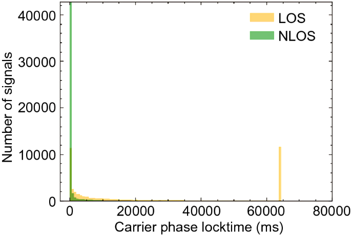

  

  The relationship between carrier phase lock-time counter and GNSS signal classification

• (ii) Pseudorange standard deviation (metres): This indicates the magnitude of the pseudorange estimation error. This value and the following two standard deviations are generated directly from the U-blox receiver. The relationship between this QI and LOS/NLOS signals is shown in Fig. 11. Almost all LOS signal values of pseudorange standard deviation were concentrated at 10.24 m. However, for NLOS signals, 15,670 values were 20.48 m (1694 for LOS signals), 4001 values were 40.96 m (129 for LOS signals), 856 values were 81.92 m (41 for LOS signals), and 36 values were even as high as 163.84 m (5 for LOS signals). The experiment shows that this QI is the most effective for LOS/NLOS classification.

  Fig. 11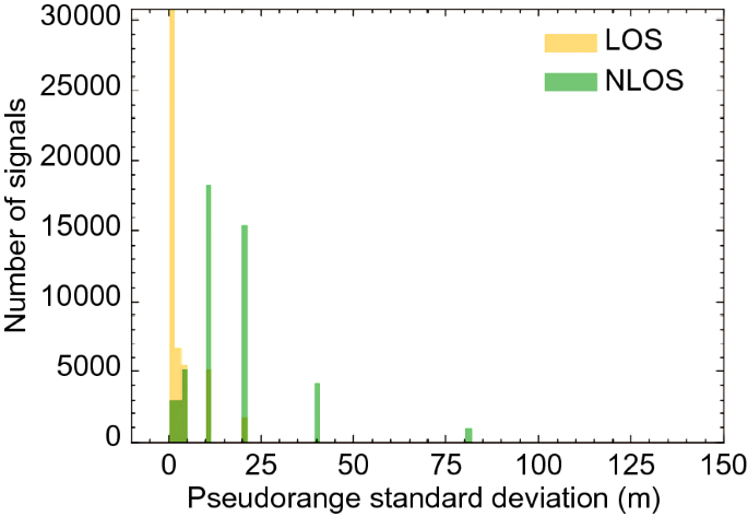

  

  The relationship between pseudorange standard deviation and GNSS signal classification

• (iii) Phase standard deviation (cycles): This indicates the magnitude of the carrier phase estimation error. The relationship between this QI and LOS/NLOS signals is shown in Fig. 12. Similar to the pseudorange standard deviation, the magnitude of the phase standard deviation of the NLOS signals is relatively large. More than 30,000 NLOS signals have the largest phase standard deviation. However, for LOS signals, the amount does not decrease monotonically as the phase standard deviation increases. 9.33% of LOS signals still have the largest phase standard deviation. Thus, this QI may not be as effective as the former QIs for classification.

  Fig. 12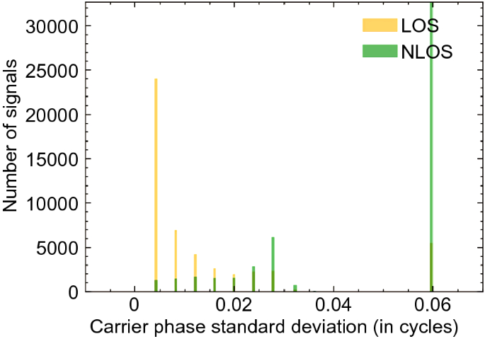

  

  The relationship between carrier phase standard deviation and GNSS signal classification

  Fig. 13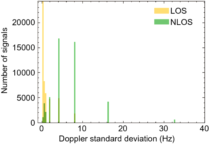

  

  The relationship between doppler standard deviation and GNSS signal classification

• (iv) Doppler standard deviation (Hertz): The Doppler shift is the carrier-phase time derivative. The U-blox receiver also estimated the Doppler standard deviation. According to the relationship between this QI and GNSS signal classification, most LOS signals have a Doppler standard deviation of less than 3 Hz, and the Doppler standard deviation of most NLOS signals is between 4 and 9 Hz (Fig. 13).

• (v) C/N₀ (decibel Hertz): Carrier-power-to-Noise-density ratio (C/N₀) indicates the signal strength of the received GNSS signal and can be used for channel scheduling and code and phase lock checking (Pini, Falletti & Fantino, 2008). It is commonly used to estimate signal quality. Yozevitch et al., (2012, 2016) set a 37 dB·Hz C/N₀ threshold to classify LOS and NLOS signals with 71% classification accuracy. The relationship between this QI and LOS/NLOS signals is shown in Fig. 14. When the C/N₀ value is small, there is a high probability that the signal is NLOS. In contrast, the LOS signal has a large C/N₀ value. There is an overlap when the C/N₀ value is between 20 and 50 dB·Hz. This overlap width is a key criterion for determining the GNSS receiver’s quality (Irish et al., 2014b). A C/N₀ mask is commonly set in the pre-processing step to exclude possible faulty signals. However, many NLOS signals tend to remain undetected in the built environment. Figure 15 shows the relationship between the C/N₀ values and the ratio of NLOS signals. Although the signal's C/N₀ is equal to 30 dB·Hz, more than 70% of the signals are NLOS. Therefore, the signal quality cannot be estimated by C/N₀ only.

  Fig. 14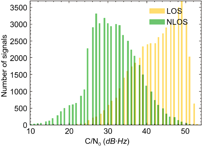

  

  The relationship between C/N₀ and GNSS signal classification

  Fig. 15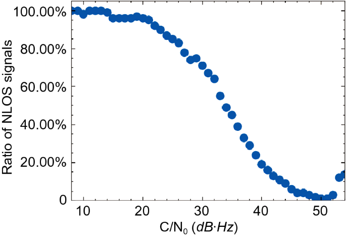

  

  The relationship between C/N₀ and the ratio of NLOS signals

  Normally, the ratio of NLOS signals decreases with an increase in C/N₀. However, a special circumstance is when the value of the C/N₀ is greater than 50 dB·Hz with an increased ratio of NLOS signals. This is because constructive multipath interference can also cause an increase in C/N₀ (Ward, 1997).

• (vi) Elevation angle (degrees): This is the angle between the line of sight and the horizontal plane, measured in the vertical plane. Like C/N₀, the elevation angle mask is also set in the pre-processing step to exclude possible outlying signals for two main reasons. First, the magnitude of the atmospheric delay error is determined by the elevation angle of the signal. Thus, the elevation angle is the variable of empirical ionospheric and tropospheric correction models. Moreover, the GNSS signals with small elevation angles can be blocked or reflected when a vehicle moves in the urban canyon. The signals with relatively large elevation angles are most likely LOS. However, in the urban canyon, the signals in the front and rear directions of the vehicle are not prone to be obstructed. On the other hand, signals received from both sides of the vehicle are easily affected by the high-rise buildings. Therefore, angle-related QIs need to be analysed comprehensively.

  The relationship between the elevation angle and LOS/NLOS signals is shown in Fig. 16. 69.80% of LOS and 19.10% of NLOS signals had more than 40 degrees elevation angles. Compared with the C/N₀, the distributions of the two signal categories concerning the elevation angle overlapped with a smaller area. This result means that the elevation angle is more feature-important for signal classification than the C/N₀. The relationship between the elevation angle and the ratio of NLOS signals is shown in Fig. 17. Similar to the C/N₀, in the urban canyon, simply setting an elevation angle mask in the pre-processing step is insufficient to exclude most NLOS signals.

  Fig. 16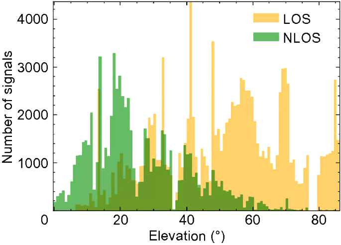

  

  The relationship between elevation angle and GNSS signal classification

  Fig. 17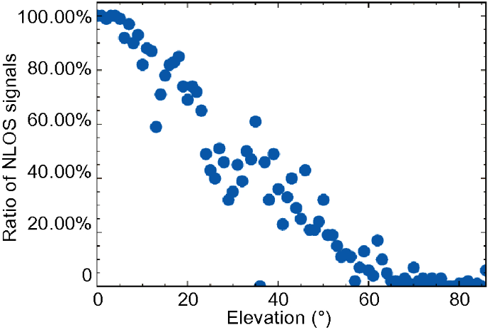

  

  The relationship between elevation angle and ratio of NLOS signals

• (vii) Azimuth (degrees): This is the angle between a GNSS satellite and the North. It is measured clockwise around the antenna's horizon or earth station's horizontal plane. A separate analysis of the azimuth angle shows no obvious relationship between this QI and GNSS signal classification (shown in Fig. 18). This result is reasonable since the GNSS satellites are scattered in all directions. However, when a vehicle moves in the urban canyon, the signals in the front and rear directions of the vehicle are not prone to be blocked or reflected. In addition, the signals received on both sides are heavily affected by high-rise buildings. Figure 9 also proves that signals on both sides of the driving direction are more likely to be NLOS. Thus, the angle between two vectors and the GNSS signal classification must be related. The two vectors are those of the azimuth angle and the vehicle's heading angle. The angle range is [0°, 90°]. We denote this angle as a difference from the azimuth angle. The relationship between this angle and GNSS signal classification is shown in Fig. 19. Compared to the NLOS signals, the LOS signals have smaller differences in azimuth angle.

  Fig. 18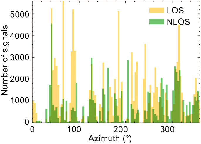

  

  Relationships between azimuth angle and GNSS signal classification

  Fig. 19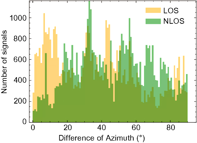

  

  Relationships between the difference in azimuth angle and GNSS signal classification

• (viii) Velocity (metres per second), acceleration (metres per second squared), and yaw rate (degrees per second): These are all vehicle-based QIs. Results show no relationship between these three QIs and GNSS signal classification. Indeed, these QIs cannot be used in a single traffic scenario to estimate the signal quality. However, in future studies, all traffic scenarios should be analysed comprehensively. In different traffic scenarios, the driving speed and yaw rate, as well as the acceleration pattern, will be different. For example, the speed limit in the United Kingdom may vary by vehicle type. For cars and motorcycles, the maximum speeds of vehicles travelling in built-up areas and motorways are 30 and 70 miles per hour, respectively. Thus, these QIs can effectively assist the system in determining the current traffic scenario and further assessing the signal quality.

• (ix) Change rate of C/N₀ (decibel Hertz): This is the difference in the C/N₀ of two adjacent time points of the same signal. Figure 20 shows that this QI is irrelevant to signal classification.

  Fig. 20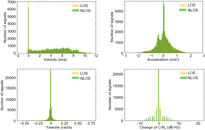

  

  The relationship between velocity, acceleration, yaw rate, or change rate of C/N₀ and GNSS signals

• (x) Measurement residual (metres): This is the difference between the pseudorange and computed range from a GNSS satellite to the estimated receiver position. In addition to GNSS signal quality, measurement residuals are also affected by the positioning method and all measurements used at that time. The results from the experiment show some residual outliers causing this QI's normal values to be closer to zero after normalisation.

  Adopting basic and weighted least squares methods with weighting schemes from (i) to (vii) in Table 2, the relationship between the measurement residual and GNSS signal classification in the same GPS time interval is shown in Fig. 21. Three findings arise from this Figure. Firstly, the distributions of LOS and NLOS signals almost completely overlap. Therefore, it is difficult to distinguish between two categories of signals using this QI alone. Secondly, the relationships vary with weighting schemes. There is, therefore, no generalised conclusion that measurement residuals obtained by a specified weighting scheme can best be used to accomplish signal classification. Finally, LOS signals tend to have greater measurement residual in the urban canyon. For example, as shown in Fig. 21 (vii), the mean values of LOS and NLOS signals are − 19.34 and − 15.18 m, with corresponding standard deviations of 23.46 and 24.40 m.

  Fig. 21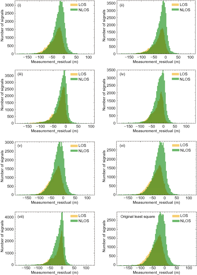

  

  Relationships between measurement residual and GNSS signal classification in different weighting schemes

  In addition, as the pseudorange residual is obtained after positioning, while signal FDE is conducted during pre-processing, this QI is not available for classification at this stage. So instead, we use the standard deviation of pseudorange to describe its error characteristics.

• (xi) Change rate of pseudorange (metres): This QI can also be used to describe the error characteristics of the pseudorange. However, it has the same drawback as the measurement residual. The outlier of this QI can be extremely large with either LOS or NLOS signals. The maximum absolute values for LOS and NLOS signals from the experiment are 175,359.78 m and 508,235 m, respectively. There are 82.66% LOS and 86.72% NLOS signals with less than 100 m of this QI. After feature normalisation, the outliers caused most values of the QI to be closer to zero. Therefore, this QI is also not recommended for classification.

  In summary, eleven QIs are discussed in this section, with the first seven shown to be important features for distinguishing LOS and NLOS signals. Therefore, the seven QIs are used in this paper as inputs to the machine learning algorithms to predict the NLOS probability of each signal.

Results of LOS/NLOS classification using machine learning algorithms

After collecting and generating all QIs needed and combining them with LOS/NLOS labels, one machine-learning dataset from four sub-datasets in Berlin and Frankfurt was created. 50,000 LOS and 50,000 NLOS signals were chosen randomly to avoid the data imbalance issue. The dataset is randomly divided into training, validating and testing sub-datasets. The ratios of the training, validating and testing sub-datasets are 52.5%, 17.5% and 30%, respectively. This section focuses on the classification results using this dataset. Ten regression algorithms are implemented to predict the NLOS probability, and then the signals are classified as LOS or NLOS by comparing the possibility to a pre-set threshold. This paper sets the threshold as 50%. This threshold is sensitive to the number of signals (e.g. in a multi-constellation scenario), measurement redundancy and LOS/NLOS trade-off.

Normally, the elevation angle and C/N₀ masks are set to exclude possible outlying signals in the GNSS processing software. This approach can be regarded as a simple decision tree model. The relationships between the two QIs and the ratio of NLOS signals were separately presented in Figs. 14 and 16. Table 4 shows the results (classification accuracy and false positives) for different elevation angles and C/N₀ masks. Note that the C/N₀ mask of 37 dB·Hz in the last row of Table 4 was proposed by Yozevitch et al., (2012, 2016).

Table 4 Classification results when setting two masks

It can be seen from Table 4 that classification accuracy increases with increasing magnitudes of the two masks while false positives decrease. This result suggests that larger masks could be effective for excluding NLOS signals. However, there are two drawbacks to this decision tree model. One is that the classification accuracy is still lower than the results of the previous studies. Compared with directly setting two thresholds, the fifteen-layer decision tree training with these two QIs achieves up to 85.95% classification accuracy and 8.19% false positive. The first three layers of the ten-layer decision tree are shown in Fig. 22, where labels 0 and 1 represent LOS and NLOS, respectively.

Fig. 22

First three layers of the ten-layer decision tree with C/N₀ and elevation angle

The second drawback is that the number of data points labelled NLOS and excluded increased with two masks. For four sets of masks in Table 4, the number of signals excluded is 4.78%, 11.49%, 20.46%, and 44.71%, respectively. The proportions of NLOS in these excluded signals are 12.21%, 25.13%, 44.67%, and 78.39%, respectively. When the elevation angle and C/N₀ masks were set to 20° and 37 dB·Hz, 9.66% of LOS signals were excluded. The remaining number of signals needs to be higher to be useful for positioning and integrity monitoring. For the decision tree model, 38.36% of signals are excluded, of which 94.14% were NLOS. This result suggests that implementing machine learning algorithms can improve classification accuracy and ensure that as many LOS signals as possible remain.

According to the previous research, two QI sets are mainly used, which are (i) elevation angle and C/N₀, (ii) the elevation angle, C/N₀, and measurement residual. These QI sets are listed in Table 5. This paper used the (vii) weighting scheme in Table 2 to calculate the measurement residual. The machine learning algorithms mainly implemented in the previous research were the SVR, KNN, GBDT, and decision tree. Moreover, the random forest method is also implemented as a bagging method. The random forest algorithm performs best in any set of QIs.

Table 5 Description of all QI sets

Moreover, the experimental results show that even though the measurement residual is not an effective QI for signal classification, this additional QI improves both classification accuracy and false positives. Therefore, in this paper, we replace the measurement residual with the pseudorange standard deviation to describe the error characteristics of the pseudorange. The third QI set (iii) comprises the elevation angle, C/N₀, and standard deviation of pseudorange. The results show that the classification accuracy is improved further. Therefore, the pseudorange standard deviation is more suitable than the pseudorange residual for LOS/NLOS classification (Table 6).

Table 6 Classification results with three sets of QIS

As discussed in the last section, seven QIs, which are carrier phase lock-time counter, pseudorange standard deviation, phase standard deviation, doppler standard deviation, C/N₀, elevation angle, and difference of azimuth angle, are combined to form the fourth (iv) set to classify LOS and NLOS signals. The classification results of ten machine learning algorithms are listed in Table 7. In this case, the performance of the bagging algorithms is better than the boosting algorithms, and the random forest method performs best. As a result, the classification accuracy of random forest methods improves from 92.20% to 93.02%, and the false positive performance improves from 3.40 to 3.01%.

Table 7 Classification results with (IV) QI set

The feature importance of all QIs fed into the random forest model is calculated and shown in Fig. 23. The standard deviation of pseudorange, C/N₀, elevation angle, and difference of azimuth angle are the first four important QIs to classify GNSS signals. The difference in azimuth angle turns out to be more important than the C/N₀ in the urban canyon. Correspondingly, the other three QIs are less important. The feature importance of each of these three QIs is less than 0.05. Some studies have already shown that using only the best features can improve the model's performance (Dewi & Chen, 2019; Jaiswal & Samikannu, 2017). Discarding less important features is more reliable, cost-effective, and time-effective. It is also important in navigation missions since the Time to Alert (TTA) should be met.

Fig. 23

Feature importance of qis in random forest

The fifth QI set (v), comprising these first four important QIs, is fed into the machine learning algorithms. The results show that the classification accuracy of the random forest model improves from 93.06% to 93.43%, and false positives decrease from 3.01% to 2.81% (Table 8). The other two algorithms, GBDT and Bagging, perform well in the classification task. One decision tree in the random forest model is shown in Fig. 24.

Fig. 24

First three layers of a decision tree in the random forest with (v) QI set

With 93.43% classification accuracy, most NLOS signals can be detected and excluded in the pre-processing step. Figure 25 illustrates the frequency plots of the number of NLOS signals at one GPS second before and after NLOS signal exclusion. Without signal exclusion, many received NLOS signals affect positioning accuracy. Therefore, multiple failures should be detected in integrity monitoring. However, after the NLOS signals are detected and excluded by the random forest algorithm, the frequency of only one NLOS signal in the signal set at one GPS second is 15.28%. The frequency of more than one NLOS signal is less than 2%.

Fig. 25

Frequency plot of the number of NLOS signals at one GPS time before or after NLOS signal exclusion

However, after NLOS signal detection and exclusion using the random forest algorithm with the (v) QI set, 41.43% of signals are excluded, of which 8.86% are LOS. For example, if seven measurements are needed for positioning at every GPS second, then there are no sufficient signals for 11.19% of the time. One possible solution to this issue is to select the seven measurements with the lowest NLOS probability values. As shown in Table 9, the GPS 16th, 18th, 26th, 27th, and GLONASS 4th and 5th signals are labelled as LOS. These six signals are insufficient for positioning. Thus, the seventh signal, the GPS 21st signal with 50.36% NLOS probability, is also selected. The NLOS impact can be mitigated with the proposed weighting scheme.

Table 8 Classification results with (V) QI set

Table 9 GNSS signal reception at one GPS second

Classification accuracy and false positives vary when setting different thresholds of NLOS probability. Figures 26  and 27 show the results of the random forest and GBDT algorithms. When the threshold is 0.5, classification accuracy is the highest. Moreover, false positives increase with a larger threshold. From the results, the random forest algorithm is always better than the GBDT in these two aspects.

Fig. 26

The relationship between the threshold value and classification accuracy results of Random Forest and GBDT

Fig. 27

The relationship between the threshold value and false positive results of Random Forest and GBDT

In comparing the results of our proposed classification algorithm with others proposed before in Table 10, we again demonstrate that the LOS/NLOS classification accuracy depends on the selected algorithms and QIs. With single QI, the upper bound of the classification accuracy was 80%. The GBDT or naïve threshold might be the best algorithm for single QI. As the number of features increased, the classification accuracy also increased. The QIs selected by other scholars were also related to signal strength, pseudorange, and elevation angle that can directly reflect the quality of the GNSS signal and influence on multipath. In this paper, we innovatively selected the difference between delta pseudorange and pseudorange rates to represent the surrounding environment and vehicle driving information. With the help of this feature, the classification accuracy increased by 3%.

Table 10 Comparison of classification algorithm performance

Results of weighting schemes

Since the random forest algorithm with the (v) QI set as input can classify LOS and NLOS signals with 93.62% classification accuracy and only 2.93% false positive, most NLOS signals can be detected and excluded. Therefore, this paper's second task is further to mitigate the NLOS impact with a novel weighting scheme. In Table 2, seven weighting schemes have been introduced. The positioning accuracy of seven weighted positioning algorithms is shown in Tables 11 and 12. Table 11 illustrates the positioning results with the elevation and C/N₀ masks set as 15. For Table 12, these masks are removed. It is worth mentioning that the singular matrix cannot be inverted without two masks. To solve this issue, we set these two masks as 1.

Table 11 Positioning accuracy with different weighting schemes and two masks

Table 12 Positioning accuracy with different weighting schemes and no masks

The result shows that with the two-mask set, the horizontal positioning error's smallest mean and standard deviation are obtained with the (vii) weighting scheme in Table 2, which are 7.990 and 5.371 m in the horizontal direction, 16.067 and 18.040 m in the vertical direction, and 20.448 and 18.411 m in the Three-Dimensional (3D) direction. The positioning accuracy is reduced when removing the masks. This result is obvious because only the (vii) scheme is designed using two QIs: the elevation angle and C/N₀. As the number of QIs increases, the quality of the GNSS signals can be better estimated. For high-quality signals, their values in the weight matrix are large. This paper proposes a novel weighting scheme (viii) which is designed as

$$\begin{array}{*{20}c} {\left( {1 - {\text{P}}_{NLOS} } \right) \times \exp \left( {{\text{C}}/{\text{N}}_0/10} \right) \times \sin^{2} \left( {elevation} \right)} \\ \end{array}$$

(9)

where ${\text{P}}_{NLOS}$ is the NLOS probability. When the signal is most likely NLOS, its weight value is small, and vice versa. The positioning results show that without NLOS signal exclusion, the mean value and standard deviation are 6.462 and 4.802 m in the horizontal direction, 8.754 and 9.185 m in the vertical direction, and 12.973 and 10.504 m in the 3D direction. Experiments have proved that the mean and standard deviation of the positioning error in the horizontal direction decreased by more than 10%. The mean and standard deviation of positioning error decreased by more than 35% in the vertical and 3D directions. Moreover, when removing the two masks, the positioning accuracy is also the highest among all weighting schemes. The impact of NLOS is well mitigated with the term $\left( {1 - {\text{P}}_{NLOS} } \right)$.

After NLOS signal detection and exclusion, the remaining signals are referred to as LOS_ml. The positioning accuracy is improved further using either the (vii) or (viii) weighting scheme (shown in Table 13). Compared with the positioning accuracy results using: (1) (vii) weighting scheme and no NLOS signal exclusion, (2) (viii) weighting scheme and NLOS signal exclusion, the positioning accuracy improved by 69.000% and 40.700% in the horizontal direction, 79.361% and 75.322% in the vertical direction, and 75.963% and 67.824% in the 3D direction.

Table 13 Positioning accuracy with different weighting schemes and NLOS signal exclusion

Conclusion

This paper investigates the GNSS LOS/NLOS signal classification algorithm and weighting scheme for accurate positioning. It is worth mentioning that we focus on NLOS signal detection and exclusion, as well as impact mitigation. Indeed, the GNSS signal could be blocked or reflected by buildings, walls, trees and others when the vehicle is driving in the built environment. To estimate signal quality, a richer set of QIs, including carrier-phase lock-time counter, the standard deviation of measurements, vehicle-based QIs, angle-related QIs, C/N₀, and others, are evaluated. Regression algorithms using these QIs as input are used to predict the NLOS probability of GNSS signals. With a pre-defined threshold, these signals can be labelled as LOS or NLOS. Results show that classification accuracy could reach 93.430%, with only 2.810% false positive of the data using the four most important QIs as input. The NLOS probability can also be used for signal subset selection and weighting scheme design. A novel weighting scheme is proposed to mitigate the impact of NLOS. The results show that the positioning accuracy improved by 69.000% and 40.700% in the horizontal direction, 79.361% and 75.322% in the vertical direction, and 75.963% and 67.824% in the 3D direction when using the random forest algorithm and novel weighting scheme.

Since this paper used an open-source dataset, the number of data points, QIs, and the urban environment were all fixed. As future scientific research work, we will collect a dataset including more QIs and data points from more constellations and more driving scenarios in the built environment. By labelling all driving scenarios, the performance of the LOS/NLOS classification algorithms can be compared and analysed thoroughly. Furthermore, the reduced number of GNSS signals every second might cause a greater Dilution of Precision (DOP) value, and then the poor satellite geometry would cause lower positioning accuracy. Two possible solutions can address this issue. (i) Collecting data from four global constellations and some regional constellations. (ii) Remaining more signals by adjusting the LOS/NLOS threshold. Correcting and excluding the NLOS signals as much as possible under the condition of the DOP and further improving the positioning accuracy will be the focus of future work. To test the performance of LOS/NLOS classification algorithms, pseudorange positioning was used in this paper. For real-time vehicle positioning, higher accuracy algorithms are always chosen, such as Real-Time Kinematic (RTK), Precise Point Positioning (PPP), and GNSS/INS integration. Research is ongoing on these positioning algorithms and relevant NLOS impact mitigation.

References

Adjrad, M., & Groves, P. D. (2017). Enhancing least squares GNSS positioning with 3D mapping without accurate prior knowledge. Navigation Journal of the Institute of Navigation., 64(1), 75–91.
Breiman, L. (1996). Bagging predictors. Machine Learning., 24(2), 123–140.
Chen, C., & Zhang, X. (2010). A fast satellite selection approach for satellite navigation system. Acta Electonica Sinica., 38(12), 2887.
Chen, C. (2015). Weighted geometric dilution of precision calculations with matrix multiplication. Sensors., 15(1), 803–817.
Chen, C., Lin, J., & Lee, C. (2013). Neural network for WGDOP approximation and mobile location. Mathematical Problems in Engineering., 2013, 589.
Collins, J. P. & Langley, R. B. (1999) Possible weighting schemes for GPS carrier phase observations in the presence of multipath. In Final Contract Report for the US Army Corps of Engineers Topographic Engineering Center, no.DAAH04–96-C-0086/TCN. 98151.
Collins, M., Schapire, R. E., & Singer, Y. (2002). Logistic regression, AdaBoost and Bregman distances. Machine Learning., 48(1), 253–285.
Dewi, C., & Chen, R. (2019). Random forest and support vector machine on features selection for regression analysis. International Journal of Innovative Computing, Information Control, 15(6), 2027–2037.
Drucker, H., Burges, C. J., Kaufman, L., Smola, A., & Vapnik, V. (1996). Support vector regression machines. Advances in Neural Information Processing Systems., 9, 470.
Eslami, E., Salman, A. K., Choi, Y., Sayeed, A., & Lops, Y. (2020). A data ensemble approach for real-time air quality forecasting using extremely randomized trees and deep neural networks. Neural Computing and Applications., 32(11), 7563–7579.
Eueler, H., & Goad, C. C. (1991). On optimal filtering of GPS dual frequency observations without using orbit information. Bulletin Géodésique., 65(2), 130–143.
European Space Agency. (2013) GNSS Data Processing Volume I: Fundamentals and Algorithms.
Friedman, J. H., & Hall, P. (2007). On bagging and nonlinear estimation. Journal of Statistical Planning and Inference., 137(3), 669–683.
Ganganwar, V. (2012). An overview of classification algorithms for imbalanced datasets. International Journal of Emerging Technology and Advanced Engineering., 2(4), 42–47.
Gaudart, J., Giusiano, B., & Huiart, L. (2004). Comparison of the performance of multi-layer perceptron and linear regression for epidemiological data. Computational Statistics and Data Analysis., 44(4), 547–570.
Geurts, P., Ernst, D., & Wehenkel, L. (2006). Extremely randomized trees. Machine Learning., 63(1), 3–42.
Groves, P. D., & Adjrad, M. (2017). Likelihood-based GNSS positioning using LOS/NLOS predictions from 3D mapping and pseudoranges. GPS Solutions, 21(4), 1805–1816.
GUERMAH, B., EL GHAZI, H., SADIKI, T. & GUERMAH, H. (2018) A robust GNSS LOS/multipath signal classifier based on the fusion of information and machine learning for intelligent transportation systems. 2018 IEEE International Conference on Technology Management, Operations and Decisions (ICTMOD)., IEEE. pp.94–100.
Guo, G., Wang, H., Bell, D., Bi, Y. & Greer, K. (2003) KNN model-based approach in classification. OTM Confederated International Conferences" On the Move to Meaningful Internet Systems"., Springer. pp.986–996.
Hartinger, H., & Brunner, F. K. (1999). Variances of GPS phase observations: The SIGMA-ɛ model. GPS Solutions, 2(4), 35–43.
Hofmann-Wellenhof, B., Lichtenegger, H. & Wasle, E. (2007) GNSS–global navigation satellite systems: GPS, GLONASS, Galileo, and more. [google] Springer Science & Business Media.
Hsu, L. (2018). Analysis and modeling GPS NLOS effect in highly urbanized area. GPS Solutions, 22(1), 1–12.
Hsu, L. (2017) GNSS multipath detection using a machine learning approach. In 2017 IEEE 20th International Conference on Intelligent Transportation Systems (ITSC) (pp. 1–6), IEEE.
Hsu, L., Tokura, H., Kubo, N., Gu, Y., & Kamijo, S. (2017). Multiple faulty GNSS measurement exclusion based on consistency check in urban canyons. IEEE Sensors Journal., 17(6), 1909–1917.
Irish, A. T., Isaacs, J. T., Quitin, F., Hespanha, J. P. & Madhow, U. (2014a) Belief propagation based localization and mapping using sparsely sampled GNSS SNR measurements. In 2014a IEEE international conference on robotics and automation (ICRA) (pp.1977–1982), IEEE.
Irish, A. T., Isaacs, J. T., Quitin, F., Hespanha, J. P. & Madhow, U. (2014b) Belief propagation based localization and mapping using sparsely sampled GNSS SNR measurements. In 2014b IEEE international conference on robotics and automation (ICRA) (pp.1977–1982), IEEE.
Jaiswal, J. K. & Samikannu, R. (2017) Application of random forest algorithm on feature subset selection and classification and regression. In 2017 world congress on computing and communication technologies (WCCCT) (pp.65–68), IEEE.
Kaplan, E. & Hegarty, C. (2005) Understanding GPS: principles and applications. [google] Artech house.
Ke, G., Meng, Q., Finley, T., Wang, T., Chen, W., Ma, W., Ye, Q., & Liu, T. (2017). Lightgbm: A highly efficient gradient boosting decision tree. Advances in Neural Information Processing Systems., 30, 4105.
Li, F., Dai, Z., Li, T. & Zhu, X. (2022) GNSS NLOS signals identification based on deep neural networks. 4th International Conference on Information Science, Electrical, and Automation Engineering (ISEAE 2022) (pp.160–169). SPIE.
Li, Z., Chen, W., Ruan, R., & Liu, X. (2020). Evaluation of PPP-RTK based on BDS-3/BDS-2/GPS observations: A case study in Europe. GPS Solutions, 24(2), 1–12.
MacGougan, G., Lachapelle, G., Klukas, R., Siu, K., Garin, L., Shewfelt, J., & Cox, G. (2002). Performance analysis of a stand-alone high-sensitivity receiver. GPS Solutions, 6(3), 179–195.
Martínez-Muñoz, G., & Suárez, A. (2010). Out-of-bag estimation of the optimal sample size in bagging. Pattern Recognition., 43(1), 143–152.
Meng, F., Wang, S., & Zhu, B. (2015). GNSS reliability and positioning accuracy enhancement based on fast satellite selection algorithm and RAIM in multiconstellation. IEEE Aerospace and Electronic Systems Magazine., 30(10), 14–27.
Montenbruck, O., Gill, E., & Lutze, F. (2002). Satellite orbits: Models, methods, and applications. Applied Mechanics Reviews, 55(2), B27–B28.
Mosavi, M. R. & Divband, M. (2010) Calculation of geometric dilution of precision using adaptive filtering technique based on evolutionary algorithms. In 2010 international conference on electrical and control engineering (pp.4842–4845), IEEE.
Murtagh, F. (1991). Multilayer perceptrons for classification and regression. Neurocomputing, 2(5–6), 183–197.
Myles, A. J., Feudale, R. N., Liu, Y., Woody, N. A., & Brown, S. D. (2004). An introduction to decision tree modeling. Journal of Chemometrics A Journal of the Chemometrics Society., 18(6), 275–285.
Novatel. (ed.) (2016) OEM6 Family of Receivers-Firmware Reference Manual.
Park, C. & How, J. P. (2001) Quasi-optimal Satellite Selection Algorithm for Real-time Applications1. In Proceedings of the 14th International Technical Meeting of the Satellite Division of The Institute of Navigation (ION GPS 2001) (pp.3018–3028).
Parkinson, B., Spilker, J. J., Axelrad, P. & Enge, P. (1996) GPS: Theory and Applications.
Phan, Q., Tan, S., McLoughlin, I., & Vu, D. (2013). A unified framework for GPS code and carrier-phase multipath mitigation using support vector regression. Advances in Artificial Neural Systems., 5, 21.
Pini, M., Falletti, E. & Fantino, M. (2008) Performance evaluation of C/N0 estimators using a real time GNSS software receiver. In 2008 IEEE 10th international symposium on spread spectrum techniques and applications (pp. 32–36.), IEEE.
Ray, J. K. & Cannon, M. E. (1999) Characterization of GPS carrier phase multipath. In Proceedings of the 1999 National Technical Meeting of the Institute of Navigation (pp. 343–352).
Reisdorf, P., Pfeifer, T., Breßler, J., Bauer, S., Weissig, P., Lange, S., Wanielik, G. & Protzel, P. (2016) The problem of comparable gnss results–an approach for a uniform dataset with low-cost and reference data. In Proceedings of International Conferences on Advances in Vehicular Systems, Technologies and Applications (VEHICULAR).
Reisdorf, P. & Wanielik, G. (2018) Approach for Self-consistent NLOS Detection in GNSS-Multi-constellation Based Localization. In Proceedings of the 31st International Technical Meeting of the Satellite Division of The Institute of Navigation (ION GNSS 2018) (pp. 3663–3670).
Rodriguez-Galiano, V., Sanchez-Castillo, M., Chica-Olmo, M., & Chica-Rivas, M. (2015). Machine learning predictive models for mineral prospectivity: An evaluation of neural networks, random forest, regression trees and support vector machines. Ore Geology Reviews., 71, 804–818.
Saber, A. G., Helal, A. N., Shaban, K. R., Abd Alla, K. M., Elmaged, A. E. A. A., Alaa Eldeen, A. E. M., Mostafa, A. E. E. D., Saber, O. H., Qenawy, M. M. A. & Fouly, M. E. (2021) Self-driving car-design and implementation. In The international undergraduate research conference (pp. 660–665), The Military Technical College.
SAE International. (2018) Taxonomy and Definitions for Terms Related to Driving Automation Systems for On-Road Motor Vehicles (J3016B).
Segal, M. R. (2004) Machine learning benchmarks and random forest regression.
Shokri, S., Rahemi, N., & Mosavi, M. R. (2020). Improving GPS positioning accuracy using weighted Kalman Filter and variance estimation methods. CEAS Aeronautical Journal., 11(2), 515–527.
Simon, D., & El-Sherief, H. (1995). Navigation satellite selection using neural networks. Neurocomputing, 7(3), 247–258.
Smola, A. J., & Schölkopf, B. (2004). A tutorial on support vector regression. Statistics and Computing., 14(3), 199–222.
Solomatine, D. P. & Shrestha, D. L. (2004) AdaBoost. RT: a boosting algorithm for regression problems. 2004 IEEE International Joint Conference on Neural Networks (IEEE Cat. No. 04CH37541) (pp. 1163–1168). IEEE.
Song, Y., Liang, J., Lu, J., & Zhao, X. (2017). An efficient instance selection algorithm for k nearest neighbor regression. Neurocomputing, 251, 26–34.
Sun, R., Fu, L., Wang, G., Cheng, Q., Hsu, L., & Ochieng, W. Y. (2021). Using dual-polarization GPS antenna with optimized adaptive neuro-fuzzy inference system to improve single point positioning accuracy in urban canyons. Navigation, 68(1), 41–60.
Sun, R., Wang, G., Cheng, Q., Fu, L., Chiang, K., Hsu, L., & Ochieng, W. Y. (2020a). Improving GPS code phase positioning accuracy in urban environments using machine learning. IEEE Internet of Things Journal., 8(8), 7065–7078.
Sun, R., Wang, G., Zhang, W., Hsu, L., & Ochieng, W. Y. (2020b). A gradient boosting decision tree based GPS signal reception classification algorithm. Applied Soft Computing., 86, 105942.
Sun, Y., Wong, A. K., & Kamel, M. S. (2009). Classification of imbalanced data: A review. International Journal of Pattern Recognition and Artificial Intelligence., 23(04), 687–719.
Sutton, C. D. (2005). Classification and regression trees, bagging, and boosting. Handbook of Statistics., 24, 303–329.
Suzuki, T., Kusama, K. & Amano, Y. (2020) NLOS multipath detection using convolutional neural network. In Proceedings of the 33rd International Technical Meeting of the Satellite Division of the Institute of Navigation (ION GNSS 2020) (pp. 2989–3000).
Tay, S. & Marais, J. (2013) Weighting models for GPS Pseudorange observations for land transportation in urban canyons. In 6th European workshop on GNSS signals and signal processing (pp. 4).
Teng, Y., & Wang, J. (2016). A closed-form formula to calculate geometric dilution of precision (GDOP) for multi-GNSS constellations. GPS Solutions, 20(3), 331–339.
Teng, Y., Wang, J., Huang, Q., & Liu, B. (2018). New characteristics of weighted GDOP in multi-GNSS positioning. GPS Solutions, 22(3), 1–9.
Townsend, B., Fenton, P., Van Dierendonck, K. & Van Nee, R. (1995) L1 carrier phase multipath error reduction using MEDLL technology. In Proceedings of ion GPS (pp. 1539–1544). INSTITUTE OF NAVIGATION.
Wang, E., Jia, C., Feng, S., Tong, G., He, H., Qu, P., Bie, Y., Wang, C. & Jiang, Y. (2018) A new satellite selection algorithm for a multi-constellation GNSS receiver. In Proceedings of the 31st International Technical Meeting of the Satellite Division of The Institute of Navigation (ION GNSS 2018) (pp. 3802–3811).
Wang, L., Groves, P. D., & Ziebart, M. K. (2015). Smartphone shadow matching for better cross-street GNSS positioning in urban environments. The Journal of Navigation., 68(3), 411–433.
Ward, N. (1997) Understanding GPS—Principles and Applications. Elliott D. Kaplan (Editor).£ 75. ISBN: 0–89006–793–7. Artech House Publishers, Boston & London. 1996. The Journal of Navigation. 50(1): 151–152.
Wei, M., Wang, J. & Li, J. (2012) A new satellite selection algorithm for real-time application. 2012 international conference on systems and informatics (ICSAI2012) (pp. 2567–2570). IEEE.
Wen, W. (2020) 3D LiDAR aided GNSS positioning and its application in sensor fusion for autonomous vehicles in urban canyons.
Wen, W., Zhang, G., & Hsu, L. (2020). Object-detection-aided GNSS and its integration with Lidar in highly urbanized areas. IEEE Intelligent Transportation Systems Magazine., 12(3), 53–69.
Wieser, A., & Brunner, F. K. (2000). An extended weight model for GPS phase observations. Earth, Planets and Space, 52(10), 777–782.
Wu, C., Su, W., & Ho, Y. (2010). A study on GPS GDOP approximation using support-vector machines. IEEE Transactions on Instrumentation and Measurement., 60(1), 137–145.
Xu, B., Jia, Q., Luo, Y., & Hsu, L. (2019). Intelligent GPS L1 LOS/multipath/NLOS classifiers based on correlator-, RINEX-and NMEA-Level Measurements. Remote Sensing., 11(16), 1851.
Xu, H., Angrisano, A., Gaglione, S., & Hsu, L. (2020). Machine learning based LOS/NLOS classifier and robust estimator for GNSS shadow matching. Satellite Navigation., 1(1), 1–12.
Xu, M., Watanachaturaporn, P., Varshney, P. K., & Arora, M. K. (2005). Decision tree regression for soft classification of remote sensing data. Remote Sensing of Environment., 97(3), 322–336.
Yin, L., Deng, Z., Xi, Y., Dong, H., Zhan, Z. & Gao, Z. (2013) A satellite selection algorithm for GNSS multi-system based on pseudorange measurement accuracy. In 2013 5th IEEE International Conference on Broadband Network & Multimedia Technology (pp. 165–168). IEEE.
Yozevitch, R., Moshe, B. B. & Levy, H. (2012) Breaking the 1 meter accuracy bound in commercial GNSS devices. In 2012 IEEE 27th Convention of Electrical and Electronics Engineers in Israel (pp. 1–5). IEEE.
Yozevitch, R., Moshe, B. B., & Weissman, A. (2016). A robust GNSS los/nlos signal classifier. Navigation Journal of the Institute of Navigation., 63(4), 429–442.
Zarei, N. (2014). Artificial intelligence approaches for GPS GDOP classification. International Journal of Computer Applications., 96(16), 48.
Zhu, J. (1992). Calculation of geometric dilution of precision. IEEE Transactions on Aerospace and Electronic Systems., 28(3), 893–895.
Zhu, N., Marais, J., Bétaille, D., & Berbineau, M. (2018). GNSS position integrity in urban environments: A review of literature. IEEE Transactions on Intelligent Transportation Systems., 19(9), 2762–2778.
Acknowledgements
Thanks for the open-source GNSS dataset from the Chemnitz University of Technology.
Funding
This research received no specific grant from any funding agency in the public, commercial, or not-for-profit sectors.
Author information
Authors and Affiliations
Contributions
LL designed and conducted the experiments and wrote the paper; ME and YF assisted in code debugging and model tuning; WYO helped with constructive guidance and revisions. All authors have read and approved the final manuscript.
Corresponding author
Ethics declarations
Competing interests
The authors declare that they have no competing interests.
Additional information
Publisher's Note
Springer Nature remains neutral with regard to jurisdictional claims in published maps and institutional affiliations.
Rights and permissions
Open Access This article is licensed under a Creative Commons Attribution 4.0 International License, which permits use, sharing, adaptation, distribution and reproduction in any medium or format, as long as you give appropriate credit to the original author(s) and the source, provide a link to the Creative Commons licence, and indicate if changes were made. The images or other third party material in this article are included in the article's Creative Commons licence, unless indicated otherwise in a credit line to the material. If material is not included in the article's Creative Commons licence and your intended use is not permitted by statutory regulation or exceeds the permitted use, you will need to obtain permission directly from the copyright holder. To view a copy of this licence, visit http://creativecommons.org/licenses/by/4.0/.
About this article
Cite this article
Li, L., Elhajj, M., Feng, Y. et al. Machine learning based GNSS signal classification and weighting scheme design in the built environment: a comparative experiment. Satell Navig 4, 12 (2023). https://doi.org/10.1186/s43020-023-00101-w
Received:
Accepted:
Published:
DOI: https://doi.org/10.1186/s43020-023-00101-w